Download

1 / 63
1.12k likes | 1.85k Vues
The Elements of Statistical Learning. Thomas Lengauer, Christian Merkwirth using the book by Hastie, Tibshirani, Friedman. Prerequisites: Vordiplom in mathematics or computer science or equivalent Linear algebra Basic knowledge in statistics Credits: Übungsschein, based on

E N D
The Elements of Statistical Learning Thomas Lengauer, Christian Merkwirth using the book by Hastie, Tibshirani, Friedman
Prerequisites: Vordiplom in mathematics or computer science or equivalent Linear algebra Basic knowledge in statistics Credits: Übungsschein, based on At least 50% of points in homework Final exam, probably oral Good for Bioinformatics CS Theory or Applications Time Lecture: Wed 11-13, HS024, Building 46 (MPI) Tutorial: Fri 14-16Rm. 15, Building 45 (CS Dep.)Biweekly, starting Oct. 31 The Elements of Statistical Learning
Applications of Statistical Learning Medical: Predicted whether a patient, hospitalized due to a heart attack, will have a second heart attack Data: demographic, diet, clinical measurements Business/Economics: Predict the price of stock 6 months from now. Data: company performance, economic data Vision: Identify hand-written ZIP codes Data: Model hand-written digits Medical: Amount of glucose in the blood of a diabetic Data: Infrared absorption spectrum of blood sample Medical: Risk factors for prostate cancer Data: Clinical, demographic
Types of Data • Two basically different types of data • Quantitative (numerical): e.g. stock price • Categorical (discrete, often binary): cancer/no cancer • Data are predicted • on the basis of a set of features (e.g. diet or clinical measurements) • from a set of (observed) training data on these features • For a set of objects (e.g. people). • Inputs for the problems are also called predictors or independent variables • Outputs are also called responses or dependent variables • The prediction model is called a learner or estimator (Schätzer). • Supervised learning: learn on outcomes for observed features • Unsupervised learning: no feature values available
Example 1: Email Spam • Data: • 4601 email messages each labeled email (+) or spam (-) • The relative frequencies of the 57 most commonly occurring words and punctuation marks in the message • Prediction goal: label future messages email (+) or spam (-) • Supervised learning problem on categorical data: classification problem Words with largest difference between spam and email shown.
Example 1: Email Spam • Examples of rules for prediction: • If (%george<0.6) and (%you>1.5) then spam else email • If (0.2·%you-0.3 ·%george)>0 then spam else email • Tolerance to errors: • Tolerant to letting through some spam (false positive) • No tolerance towards throwing out email (false negative) Words with largest difference between spam and email shown.
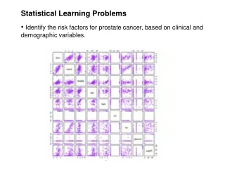
Example 2: Prostate Cancer • Data (by Stamey et al. 1989): • Given: lcavol log cancer volumelweight log prostate weightagelbph log benign hyperplasia amountsvi seminal vesicle invasionlcp log capsular penetrationgleason gleason scorepgg45 percent gleason scores 4 or 5 • Predict:PSA (prostate specific antigen) level • Supervised learning problem on quantitative data: regression problem
Example 2: Prostate Cancer • Figure shows scatter plots of the input data, projected onto two variables, respectively. • The first row shows the outcome of the prediction, projected onto each input variable, respectively. • The variables svi and gleason are categorical
Data: images are single digits 16x16 8-bit gray-scale, normalized for sizeand orientation Classify: newly written digits Non-binary classification problem Low tolerance to misclassifications Example 3: Recognition of Handwritten Digits
Data: Color intensities signifying the abundance levels of mRNA for a number of genes (6830) in several (64) different cell states (samples). Red over-expressed gene Green under-expressed gene Black normally expressed gene (according to some predefined background) Predict: Which genes show similar expression over the samples Which samples show similar expression over the genes (unsupervised learning problem) Which genes are highly over or under expressed in certain cancers (supervised learning problem) Example 4: DNA Expression Microarrays genes samples
Inputs X, Xj(jth element of vector X) p #inputs, N #observations Xmatrix written in bold Vectors written in bold xi if they have N components and thus summarize all observations on variable Xi Vectors are assumed to be column vectors Discrete inputs often described by characteristic vector (dummy variables) Outputs quantitative Y qualitative G(for group) Observed variables in lower case The i-th observed value of X is xi and can be a scalar or a vector Main question of this lecture: Given the value of an input vectorX, make a goodpredictionŶof the outputY The prediction should be of the same kind as the searched output (categorical vs. quantitative) Exception: Binary outputs can be approximated by values in [0,1], which can be interpreted as probabilities This generalizes to k-level outputs. 2.2 Notation
Given inputsX=(X1,X2,…,Xp) Predict outputYvia the model Include the constant variable 1 in X Here Yis scalar (If Y is a K-vector then X is apxK matrix) In the (p+1)-dimensional input-output space, (X,Ŷ ) represents a hyperplane If the constant is included in X, then the hyperplane goes through the origin is a linear function is a vector that points in the steepest uphill direction 2.3.1 Simple Approach 1: Least-Squares
In the (p+1)-dimensional input-output space, (X,Ŷ ) represents a hyperplane If the constant is included in X, then the hyperplane goes through the origin is a linear function is a vector that points in the steepest uphill direction 2.3.1 Simple Approach 1: Least-Squares b
Training procedure: Method of least-squares N = #observations Minimize the residual sum of squares Or equivalently This quadratic function always has a global minimum, but it may not be unique Differentiating w.r.t. b yields the normal equations If XTX is nonsingular, then the unique solution is The fitted value at input xis The entire surface is characterized by . 2.3.1 Simple Approach 1: Least-Squares
Example: Data on two inputs X1 and X2 Output variable has values GREEN (coded 0) and RED (coded 1) 100 points per class Regression line is defined by Easy but many misclassifications if the problem is not linear 2.3.1 Simple Approach 1: Least-Squares X1 X2
Uses those observations in the training set closest to the given input. Nk(x) is the set of the k closest points to x is the training sample Average the outcome of the k closest training sample points Fewer misclassifications 2.3.2 Simple Approach 2: Nearest Neighbors 15-nearest neighbor averaging X1 X2
Uses those observation in the training set closest to the given input. Nk(x) is the set of the kclosest points to x is the training sample Average the outcome of the k closest training sample points No misclassifications: Overtraining 2.3.2 Simple Approach 2: Nearest Neighbors 1-nearest neighbor averaging X1 X2
Least squares K-nearest neighbors 2.3.3 Comparison of the Two Approaches
Least squares p parameters p =#features K-nearest neighbors Apparently one parameter kIn fact N/k parametersN =#observations 2.3.3 Comparison of the Two Approaches
Least squares p parameters p =#features Low variance (robust) K-nearest neighbors Apparently one parameter kIn fact N/k parametersN =#observations High variance (not robust) 2.3.3 Comparison of the Two Approaches
Least squares p parameters p =#features Low variance (robust) High bias (rests on strong assumptions) K-nearest neighbors Apparently one parameter kIn fact N/k parametersN =#observations High variance (not robust) Low bias (rests only on weak assumptions) 2.3.3 Comparison of the Two Approaches
Least squares p parameters p =#features Low variance (robust) High bias (rests on strong assumptions) Good for Scenario 1:Training data in each class generated from a two-dimensional Gaussian, the two Gaussians are independent and have different means K-nearest neighbors Apparently one parameter kIn fact N/k parametersN =#observations High variance (not robust) Low bias (rests only on weak assumptions) Good for Scenario 2:Training data in each class from a mixture of 10 low-variance Gaussians, with means again distributed as Gaussian (first choose the Gaussian, then choose the point according to the Gaussian) 2.3.3 Comparison of the Two Approaches
Mixture of the two scenarios Step 1: Generate 10 means mk from the bivariate Gaussian distribution N((1,0)T,I) and label this class GREEN Step 2: Similarly, generate 10 means from the from the bivariate Gaussian distribution N((0,1)T,I) and label this class RED Step 3: For each class, generate 100 observations as follows: For each observation, pick an mk at random with probability 1/10 Generate a point according to N(mk,I/ 5) Similar to scenario 2 Result of 10 000 classifications 2.3.3 Origin of the Data
2.3.3 Variants of These Simple Methods • Kernel methods: use weights that decrease smoothly to zero with distance from the target point, rather than the 0/1 cutoff used in nearest-neighbor methods • In high-dimensional spaces, some variables are emphasized more than others • Local regression fits linear models (by least squares) locally rather than fitting constants locally • Linear models fit to a basis expansion of the original inputs allow arbitrarily complex models • Projection pursuit and neural network models are sums of nonlinearly transformed linear models
Random input vector: Random output variable: Joint distribution: Pr(X,Y) We are looking for a functionf(x)for predictingYgiven thevalues of the inputX The loss function L(Y,f(X))shall penalize errors Squared error loss: Expected prediction error (EPE): Since Pr(X,Y)=Pr(Y|X )Pr(X ) EPE can also be written as Thus it suffices to minimize EPE pointwise 2.4 Statistical Decision Theory Regression function:
Nearest neighbor methods try to directly implement this recipe Several approximations Since no duplicate observations, expectation over a neighborhood Expectation approximated by averaging over observations With increasing k and number of observations the average gets (provably) more stable But often we do not have large samples By making assumptions (linearity) we can reduce the number of required observations greatly. With increasing dimension the neighborhood grows exponentially. Thus the rate of convergence to the true estimator (with increasing k) decreases 2.4 Statistical Decision Theory Regression function:
Linear regression Assumes that the regression function is approximately linear This is a model-based approach After plugging this expression into EPE and differentiating w.r.t. b, we can solve for b Again, linear regression replaces the theoretical expectation by averaging over the observed data Summary: Least squares assumes that f(x) is well approximated by a globally linear function Nearest neighbors assumes that f(x) is well approximated by a locally constant function. 2.4 Statistical Decision Theory Regression function:
Additional methods in this book are often model-based but more flexible than the linear model. Additive models Each fj is arbitrary What happens if we use another loss function? In this case More robust than the conditional mean L1 criterion not differentiable Squared error most popular 2.4 Statistical Decision Theory
Procedure for categorical output variable G with values from G Loss function is kxk matrix L where k = card(G) L is zero on the diagonal L(k, ℓ)is the price paid for misclassifying a element from class Gkas belonging to class Gℓ Frequently 0-1 loss function used: L(k, ℓ)= 1-dkl Expected prediction error (EPE) Expectation taken w.r.t. the joint distribution Pr(G,X) Conditioning yields Again, pointwise minimization suffices Or simply Bayes Classifier 2.4 Statistical Decision Theory
Expected prediction error (EPE) Expectation taken w.r.t. the joint distribution Pr(G,X) Conditioning yields Again, pointwise minimization suffices Or simply 2.4 Statistical Decision Theory Bayes-optimal decision boundary Bayes Classifier
Curse of Dimensionality:Local neighborhoods become increasingly global, as the number of dimension increases Example: Points uniformly distributed in a p-dimensional unit hypercube. Hypercubical neighborhood in p dimensions that captures a fraction r of the data Has edge length ep(r) = r1/p e10(0.01) = 0.63 e10(0.1) = 0.82 To cover 1% of the data we must cover 63% of the range of an input variable 2.5 Local Methods in High Dimensions
To cover 1% of the data we must cover 63% of the range of an input variable 2.5 Local Methods in High Dimensions • Reducing r reduces the number of observations and thus the stability
In high dimensions, all sample points are close to the edge of the sample N data points uniformly distributed in a p-dimensional unit ball centered at the origin Median distance from the closest point to the origin (Homework) d(10,500) = 0.52 More than half the way to the boundary Sampling density is proportional toN1/p If N1 = 100 is a dense sample for one input then N10 = 10010 is an equally dense sample for 10 inputs. 2.5 Local Methods in High Dimensions 1/2 1/2 median
Another example T set of training points xi generated uniformly in [-1,1]p (red) Functional relationship between X and Y (green) No measurement error Error of a 1-nearest neighbor classifier in estimating f(0) (blue) closest training point 10 training points 2.5 Local Methods in High Dimensions prediction
Another example Problem deterministic: Prediction error is the mean-squared error for estimating f(0) downward bias telescoping closest training point 10 training points 2.5 Local Methods in High Dimensions prediction
Another example 1-d vs. 2-d Bias increases 2-d bias 1-d bias 2.5 Local Methods in High Dimensions
The case on N=1000 training points Bias increases since distance of nearest neighbour increases Variance does not increase since function symmetric around 0 2.5 Local Methods in High Dimensions Average
Yet another example Variance increases since function is not symmetric around 0 Bias increases moderately since function is monotonic 2.5 Local Methods in High Dimensions
Assume now a linear relationship with measurement error We fit the model with least squares, for arbitrary test point x0 Additional variance s2 since output nondeterministic Variance depends on x0 If N is large we get Variance negligible for large N or small s No bias Curse of dimensionality controlled Additional variance 2.5 Local Methods in High Dimensions
More generally Sample size:N = 500 Linear case EPE(LeastSquares) is slightly above 1no bias EPE(1-NN) always above 2, grows slowlyas nearest training point strays from target 2.5 Local Methods in High Dimensions EPE Ratio 1-NN/Least Squares
More generally Sample size:N = 500 Cubic Case EPE(LeastSquares) is biased, thus ratio smaller 2.5 Local Methods in High Dimensions EPE Ratio 1-NN/Least Squares
2.6 Statistical Models • NN methods are the direct implementation of • But can fail in two ways • With high dimensions NN need not be close to the target point • If special structure exists in the problem, this can be used to reduce variance and bias
Assume additive error model Then Pr(Y|X) depends only onthe conditional mean off(x) This model is a good approximation in many cases In many cases, f(x) is deterministic and error enters through uncertainty in the input. This can often be mapped on uncertainty in the output with deterministic input. 2.6.1 Additive Error Model
Supervised learning The learning algorithm modifies its input/output relationship in dependence on the observed error This can be a continuous process 2.6.2 Supervised Learning
Data: pairs (xi,yi) that are points in (p+1)-space More general input spaces are possible Want a good approximation of f(x) in some region of input space, given the training set T Many models have certain parameters E.g. for the linear model f(x)=xTb and = b Linear basis expansions have the more general form Examples Polynomial expansions: hk(x) = x1x22 Trigonometric expansionshk(x) = cos(x1) Sigmoid expansion 2.6.3 Function Approximation
Approximating f by minimizing the residual sum of squares Linear basis expansions have the more general form Examples Polynomial expansions: hk(x) = x1x22 Trigonometric expansionshk(x) = cos(x1) Sigmoid expansion 2.6.3 Function Approximation
Approximating f by minimizing the residual sum of squares Intuition f surface in (p+1)-space Observe noisy realizations Want fitted surface as close to the observed points as possible Distance measured by RSS Methods: Closed form: if basis function have no hidden parameters Iterative: otherwise 2.6.3 Function Approximation