Introduction to Image Processing (Signal Processing)

1. Introduction to Image Processing (Signal Processing) NEU 259 Gina Sosinsky May 13, 2012

2. Quantization of images is key….

3. f H0 H1 Simian SV40 Hn g The Electron Microscope(Example of a Physical System)

4. f0 g0 H0 f0 f1 gn fn Hn H0 H1 f1 g1 g0 H1 g g1 fn Hn gn f g H f g H0 H1 Systems and Signals • Physical systems can be modeled as input signals that are transformed by the system, or cause the system to respond in some way, resulting in other signals, e.g., all imaging devices.

5. What is image processing? • The analysis, manipulation, storage, and display of graphical images from sources such as photographs, drawings, and video. • Any technique either computational or photographic which alters the information in an image. • The analysis, manipulation, storage, and display of signals in a multi-dimensional space.

6. Common Topics in Image Processing • Acquisition of Images. • Representation and Storage. • Correction of Imaging Defects (Image Restoration). • Image Enhancement (Real and Reciprocal Spaces). • Image Segmentation. • Feature Recognition and Classification. • Boolean Operations. • Morphological Operations. • Image Measuring. • Three-dimensional Imaging. • Image Visualization (2D and 3D).

7. What is image processing? • Any technique either computational or photographic which alters the information in the image. • Examples • Reversing the contrast of an image (black becomes white and vice versa). • Maximizing the values for color tables (histogram stretching) • Pattern recognition & analysis (correlations). • As Misell points out, image processing will not turn a poor image into a good one, but extracts the maximum amount of structural information from the original.

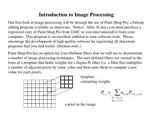
8. Types of operations an input image a[m,n] ==> an output image b[m,n] (or another representation) * Point- the output value at a specific coordinate is dependent only on the input value at that same coordinate. * Local - the output value at a specific coordinate is dependent on the input values in the neighborhood of that same coordinate. * Global - the output value at a specific coordinate is dependent on all the values in the input image.

9. Image Enhancement Objective: process an image to obtain the most information from it for a particular application. Example: Common operations to enhance images depend on the convolution of masks and the Fourier transform.

10. How do I know that my new/corrected/enhanced image is correct? • Does it resemble the original image? • Are any unusual features being introduced (e.g. aliasing)? • Is it consistent with other results outside of this image (e.g. biochemistry, NMR, MRI etc.)?

11. Two simple operations • Reversing the contrast new_pix = max - old_pix + min

12. Histogram stretching(contrast stretching) Can use histogram to replace out-lying points.

13. A bit of history • For electron micrographs, first applications: Markham et al. in 1963, Klug and Berger in 1964. • Involved the signal from a periodic specimen was separated from the non-periodic noise (electron crystallography). • Seminal publications: • Crowther, DeRosier, Klug, Nature 1968 • Unwin and Henderson, JMB 1976

14. Specific topics • Shannon sampling and Nyquist limits • Fourier analysis • Projection Theorem • Convolution theorem • Resolution & Filtering • Correlation analysis

15. Shannon Sampling & Nyquist limits Nyquist Limitis defined as 2  r/M. M = magnification; r = step size of scanner or camera Basically, the Shannon sampling theorem tells you that you need at least 2 data points to sample a function. But…in practice, in order to get a given resolution, you need to use r/(3  M) or r/(4  M) (e.g. if you want 12 Å resolution, you need to use a pixel size of 3-4 Å) This is referred to as oversampling your data. Undersampling can result in an image processing artifact known as aliasing.

16. Shannon Sampling & Nyquist Limits Effect of sampling interval on recovery of information. In this example, a sampling interval of 32 appears to be just fine enough to recover the shape of the 1D function without loss of information. At coarser sampling intervals (4-16), the subtler features in the data are lost. In practice, one aims to digitize the data at a fine enough interval to be certain that no information is lost. Thus, using the three-times pixel resolution criteria, in this example one ought to sample the data 96 (= 3 x 32) or greater to be certain to recover all the information contained in the data.

17. Raster size versus Nyquist limits

18. Jean Baptiste Joseph Fourier(1768-1830) “The profound study of nature is the most fertile source of mathematical discoveries.” Fourier Theory using trigonometrical series expansion done in ~1807 http://www-groups.dcs.st-and.ac.uk/~history/Mathematicians/Fourier.html

19. Fear not the Fourier Transform, it is your friend! Continuous FT Discrete FT (what we calculate) Inverse FT r = T-1 (T(r)) Inverse Theorem

20. Terms for Fourier analysis • Real space: Our coordinate system (x,y,z) • Reciprocal, Fourier, inverse, tranform space: Coordinate system after Fourier transformation • Amplitudes and phases or real and imaginary parts due to complex number analysis • (xyz)  Fourier transform (F (hkl)exp i(hkl)) • Where F(hkl) is the amplitude and  is the phase and • (xyz) is the density function

21. Need both phase and amplitude data correct amplitudes random phases random amplitudes correct phases Original

22. Reciprocal Space: The Final Frontier • Dimensions in the object (REAL SPACE) are inversely related to dimensions in the transform (RECIPROCAL SPACE). • Small spacings or features in real space are represented by features spaced far apart in reciprocal space. Resolution is inversely proportional to spacings. • Outer regions of the transform arise from fine (high resolution) details in the object. Coarse object features contribute near the central (low resolution) region of the transform.

23. Advantages of using Fourier analysis • The recorded diffraction pattern of an object is the square of the Fourier transform of that object. • FT are linear process (like multiplication and division). Can go backward and forward easily if functions are known. Advantages for micrographs where the FT is calculated and we want to do noise reduction, filtering or averaging. • Projection Theorem(next slides) • Convolution Theorem: Deconvolution is more easily computed in Fourier space rather than in real space (slides after Projection Theorem).

24. The Fourier Duck Behold the duck. It does not cluck. A cluck it lacks. It quacks. It is specially fond of a puddle or pond. When it dines or sups, it bottoms ups. • The Fourier Duck originated in a book of optical transforms (Taylor, C. A. & Lipson, H., Optical Transforms 1964). An optical transform is a Fourier transform performed using a simple optical apparatus. http://www.ysbl.york.ac.uk/~cowtan/fourier/fourier.html

25. The Fourier Cat and its Transform FT FT-1

26. Resolution in real versus reciprocal space The effect of taking only low angle diffraction to form the image of a duck object. A drawing of a duck is shown, together with its diffraction pattern. Also shown are the images formed (as the diffraction pattern of the diffraction pattern) when stops are used to progressively more of the high angle diffraction pattern. (From Holmes and Blow)

27. FT FT-1 FT FT-1

28. This is a test – If we take the amplitudes of the Fourier Duck and the phases of the Fourier Cat and back transform, what will we get?

29. Duck amplitudes, Cat Phases Yes, we get the Fourier Cat!

30. Projection Theorem This is the most fundamental principle for 3D reconstruction from electron micrographs. Every micrograph we obtain in TEM is a projection (sum) of everything in the specimen.

32. When examining 3D objects, 2D images may not provide the complete picture

33. The Projection Theorem Simply stated it says: The Fourier Transform of the projected structure of a 3D object is equivalent to a 2D central section of the 3D Fourier transform of the object. The central section intersects the origin of the 3d transform and is perpendicular to the direction of the projection. The 3d structure is reconstructed from several independent 2d views by the inverse Fourier transform of the complete 3d Fourier transform.

34. Radon and X-ray transforms

35. Illustration of Projection Theorem Projections Central Sections Baumeister et al. (1999) Trends Cell Biol., 9, 81-85.

36. The Convolution Theorem The convolution theorem is one of the most important relationships in Fourier theory It forms the basis of X-ray, EM and neutron crystallography.

37. Holmes and Blow (1965) give a general statement of the operation of convolution of two functions: "Set down the origin of the first function in every possible position of the second, multiply the value of the first function in each position by the value of the second at that point and take the sum of all such possible operations." c(u) = f(x) * g(x) Convolution symbol Also use 

38. Properties of Convolution • Convolution is commutative. • c = a * b = b * a • Convolution is associative. • c = a * (b * d) = (a * b) * d = a * b * d • Convolution is distributive. • c = a * (b + d) = (a * b) + (a * d) • where a, b, c, and d are all images, either continuous or discrete.

39. A simple example of convolution. One function is a drawing of a duck, the other is a 2D lattice. The convolution of these functions is accomplished by putting the duck on every lattice point. (From Holmes and Blow, p.123)

40. FT FT-1 Molecule convoluted with lattice points FT FT-1

41. Convolution & Fourier Transforms • Fourier transform of the convolution of two functions is the product of their Fourier transforms. T(ƒ *g) = F x G • The converse of the above also holds, namely that the Fourier transform of the product of two functions is equal to the convolution of the transforms of the individual functions. T(ƒ x g) = F * G Computationally, multiplication and fast-Fourier transform algorithms are speedier processes than deconvolution.

42. Words to image process by Convolution is easy, Deconvolution is hard. (Thursday’s lecture) Need to know: T(ƒ x g) = F * G

43. Simple Filtering Operations • Low pass filter • High pass filter • Band pass filter • Crystalline masks, Layer line masks (All the above can have hard or soft edges) • Median filter • Sobel filter • Rotational harmonics filtering (Fourier-Bessel analysis)

44. The Fourier Duck

45. The Fourier Duck: Low pass filtering • If we only have the low resolution terms of the diffraction pattern, we only get a low resolution duck:

46. High pass filtering • If we only have the high resolution terms of the diffraction pattern, we see only the edges of the duck but see internal features (missing box function):

47. Inverse band pass (missing shell of data) • The edges are sharp, but there is smearing around them from the missing intermediate resolution terms. The core of the duck is at the correct level, but the edges are weak.

48. Hard versus soft edged filters • Gaussian falloffs at the edges prevent aliasing artifacts. • Butterworth filters also have soft edges Butterfield Gaussian

49. Crystalline masking

50. Median Filter (Real space filter based on image statistics) • Ranks the pixels in a neighborhood (kernel) according to their brightness value (intensity). The median value in the ordered list is used as a brightness value for the central pixel. • Excellent rejector of “shot noise” and for smoothing operations. Outlying pixels are replaced by a reasonable value -- the median value in the neighborhood.