Nonparametric tests

1. Nonparametric tests Dr William Simpson Psychology, University of Plymouth

2. Hypothesis testing

3. An experiment • Volunteers sign up to weight loss expt • Randomly assign half to low carb diet, • half to low fat diet • For each subject, find weight loss at end • Low carb (C): 10,6,7,8,14 kg • Low fat (F): 5,1,3,9,2 kg

4. Is it “significant”? • We have: • C<-c(10,6,7,8,14); mean(C) is 9 • F<-c(0,1,3,9,2); mean(F) is 3 • It’s obvious that low carb works better for these subjects • Statistical significance comes in when we want to talk about people in general or if we were to repeat the expt or if we wonder if low fat diet “really works”

5. Hypothesis testing • A random process was involved with these data: random assignment • Suppose that each person would lose the same am’t of weight regardless of diet: • 10,6,7,8,14,0,1,3,9,2 • By chance, the big weight losers were assigned to the low carb diet and low ones to low fat • How likely is this sceptical idea?

6. Argument by contradiction • Assume the opposite of what we want to show (“A”) • Show that this assumption leads to absurd conclusion • Therefore initial assumption was wrong; conclude “not A”

7. Guy at party asserts: “solids are denser than liquids” • I disagree. I want to show that liquids can be denser • Assume the opposite of what I want to show: solid H2O is denser than liquid • If ice were denser, then it would sink in water • Ice does not sink • Therefore ice is less dense than water

8. Null hypothesis testing • Assume the opposite of what we want to show: Pattern of weight loss just due to random assignment • Show that this assumption leads to very unlikely conclusion • Therefore initial assumption was wrong; weight loss NOT just random assignment (ie due to diet)

9. Weight loss hypo testing • Null hypo: Pattern of weight loss just due to random assignment • Calculate a “test statistic” • Find prob of getting such an extreme test statistic if null hypo is true • If prob is low, reject null hypo. The difference is “statistically significant”

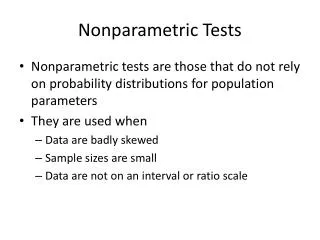
10. “Nonparametric” tests • Some types of statistical test make assumptions about the data distribution (e.g. Normal) • Nonparametric tests make no such assumptions

11. When useful? • Interval or ratio data but don’t want to make assumption about distribution and small sample size • Ordinal (rank) data

12. Ordinal data • Data in graded categories. E.g. Likert scale: • Strongly disagree • Disagree • Neither agree or disagree • Agree • Strongly Agree

13. The tests

14. 1. Two independent groups, between subjects

15. a) Permutation test • In weight loss expt, each subject assigned randomly to one of two groups • Null hypo says that our data are due simply to a fluke of random assignment

16. Permutation test: use computer to do many random permutations. Compute diff in means each time. Get distrib. See how likely it is to get diff as big as ours: • mean(C) – mean(F) = 9-3 =6kg

17. What mean diff C-F should we get if just random assignment? • Should be near zero, but will vary.

18. C:(10,6,7,8,14) F:(0,1,3,9,2) • diff • 9 6 3 1 0 2 14 7 10 8 -4.4 • 2 6 8 10 7 14 0 9 3 1 1.2 • 7 3 9 14 0 6 10 1 8 2 1.2 • 14 0 1 6 9 10 8 2 7 3 0.0 • … 1000s of times

19. C<-c(10,6,7,8,14) • F<-c(0,1,3,9,2) • x<-c(C,F) • nsim<-5000 • d<-rep(0,nsim) • for (i in 1:nsim) • { • samp<-sample(x) • d[i]<-mean(samp[1:5])-mean(samp[6:10]) • }

20. hist(d)

21. P(diff>=6)=.01 • sum(d>=6)/nsim

22. If null hypo is true, chance of getting as big a mean diff as we found (6 kg) or bigger is about .01 • This is a “low” prob. Conventional low probs are .05, .01, .001

23. Reject null hypo. Diff in weight loss not just due to random assignment. Statistically significant (p=.01) • “Those on the low-carb diet lost significantly less weight (permutation test, p=.01)”

24. Why do we say “p of getting diff as big as we got or bigger”? • Because we would also reject null if we had diff bigger than 6

25. Tails

26. One-tailed • If we predicted that low fat would work better, expect mean(C) – mean(F) >0 • What is chance of getting C-F=6 or more?

27. P(diff>=6) is right-hand • tail

28. Two-tailed • Reviewer says: “Yeah, but it could have turned out the other way, with C-F<0. You should have tested for both possibilities”

29. Can test both possibilities at same time. • Reject null either if C-F is a big negative or a big positive diff. • Both tails of distribution.

31. One-tailed or directional test: p=.0142 • sum(d>=6)/length(d) • Two-tailed or nondirectional test: p=.034 • sum(d>=6)/length(d) + sum(d<= -6)/length(d)

32. One- vs two-tailed • The p-value for 2-tailed will always be about twice as big as for 1-tailed • Harder to get statistical signif • More convincing to reviewers

33. Fallibility of hypo tests • When p-value is small (<.05), we reject null hypo • BUT 5 times in 100, null hypo will actually be true! Type I error

34. Also possible to get a big p-value and fail to reject null even if a real effect exists. Type II error • Will happen if effect is small and if sample size is small. Low power

35. b) Mann-Whitney-Wilcoxon test • Suppose that we lump all the scores together • C:(10,6,7,8,14) F:(0,1,3,9,2) • c,c,c,c,c,f,f,f,f,f • 10,6,7,8,14,0,1,3,9,2

36. Now rank these scores • If the diet had no effect on weight loss, expect the average of the ranks associated with the Fs and with the Cs to be similar.

37. Pretend we originally had • 0 7 10 8 2 9 3 1 6 14 • Ranks: • 1 6 9 7 3 8 4 2 5 10 • mean(0,7,10,8,2)=5.2 mean(9,3,1,6,14)=5.8

38. If the diet had an effect, expect the mean of the ranks assoc with F to be markedly different from the mean of the ranks assoc with C.

39. Pretend we originally had • 0 1 2 3 6 7 8 9 10 14 • Ranks: • 1 2 3 4 5 6 7 8 9 10 • mean(0,1,2,3,6)=2.4mean(7,8,9,10,14)=9.6

40. Thus, if the average (or sum*) of the ranks associated with the Cs or Fs is too large or small, we have evidence that the null (weight loss same in both) should be rejected • *mean=sum/n, so same except for scale factor

41. Weight loss example • Low carb (C): 10,6,7,8, 14 • Low fat (F): 0, 1,3,9,2 Score Rank Group 14 10 C 10 9 C 9 8 F 8 7 C 7 6 C 6 5 C 3 4 F 2 3 F 1 2 F 0 1 F Sum of ranks for Group C= 10 + 9 + 7 + 6 + 5 = 37 Sum of ranks for Group F = 8 + 4 + 3 + 2 + 1 = 18

42. Using the summed ranks, calculate a statistic (Mann-Whitney U) • Distribution of U has been tabulated, given sample sizes n1 and n2 • Look up p-value in table

43. wilcox.test() Performs one- and two-sample Wilcoxon tests on vectors of data; the latter is also known as ‘Mann-Whitney’ test. • wilcox.test(C,F,alternative="greater") • Wilcoxon rank sum test • data: C and F • W = 22, p-value = 0.02778 • alternative hypothesis: true location shift is greater than 0

44. wilcox.test(C,F,alternative="two.sided") • Wilcoxon rank sum test • data: C and F • W = 22, p-value = 0.05556 • alternative hypothesis: true location shift is not equal to 0

45. Note: different tests • Not all tests give the same answers • The permutation test gave smaller p-value (p=.034) than the U test (p=0.056) • Which one to believe? Use judgement

46. 2. Paired groups, repeated measures, within subjects

47. Repeated measures design • Repeated measures: each subject participates in conditions in random order • Each subject serves as own control • Data to be used: differences between each pair of scores.

48. a) Permutation test • Use computer to re-assign order many times. Each time find mean of the diffs. Distribution of these gives prob of getting mean diff as big as we observe

49. Null hypo: each person has a pair of scores, emitting one the first time tested and the other the 2nd time tested. These scores not related to treatment (C or F)

50. Randomly shuffle the scores. Find mean diff each time. • At end, have distrib of mean diffs