Download
1 / 58
580 likes | 589 Vues
A Study on Parallelization of Successive Rotation Based Joint Diagonalization. Xiu-Lin Wang, Xiao-Feng Gong, Qiu-Hua Lin Dalian University of Technology, China 19 th DSP, August, 2014. Content. 1. Introduction 2. The successive rotation 3. The proposed algorithm 4. Simulation results

E N D
A Study on Parallelization of Successive Rotation Based Joint Diagonalization Xiu-Lin Wang, Xiao-Feng Gong, Qiu-Hua Lin Dalian University of Technology, China 19th DSP, August, 2014
Content • 1. Introduction • 2. The successive rotation • 3. The proposed algorithm • 4. Simulation results • 5. Conclusion 1
1. Introduction JD seeks unloading matrix so that are diagonal Joint diagonalization Target matrices …… 2
1. Introduction • Joint Diagonalization(JD) has been widely applied • Array processing (X. F. Gong, 2012) • Tensor decomposition (L. Delathauwer, 2008; X. F. Gong, 2013) • Speech signal processing (D. T. Pham, 2003) • Blind source separation (J. F. Cardoso, 1993; A. Mesloub, 2014) Slicewise form: Fig.1 Visualization of models for CPD 3
1. Introduction • Joint Diagonalization(JD) has been widely applied • Array processing (X. F. Gong, 2012) • Tensor decomposition (L. Delathauwer, 2008; X. F. Gong, 2013) • Speech signal processing (D. T. Pham, 2003) • Blind source separation (J. F. Cardoso, 1993; A. Mesloub, 2014) Slicewise form: Fig.1 Visualization of models for CPD 3
1. Introduction • Joint Diagonalization(JD) has been widely applied • Array processing (X. F. Gong, 2012) • Tensor decomposition (L. Delathauwer, 2008; X. F. Gong, 2013) • Speech signal processing (D. T. Pham, 2003) • Blind source separation (J. F. Cardoso, 1993; A. Mesloub, 2014) Slicewise form: Fig.1 Visualization of models for CPD 3
1. Introduction • Joint Diagonalization(JD) has been widely applied • Array processing (X. F. Gong, 2012) • Tensor decomposition (L. Delathauwer, 2008; X. F. Gong, 2013) • Speech signal processing (D. T. Pham, 2003) • Blind source separation (J. F. Cardoso, 1993; A. Mesloub, 2014) Slicewise form: Fig.1 Visualization of models for CPD 3
1. Introduction • Joint Diagonalization(JD) has been widely applied • Array processing (X. F. Gong, 2012) • Tensor decomposition (L. Delathauwer, 2008; X. F. Gong, 2013) • Speech signal processing (D. T. Pham, 2003) • Blind source separation (J. F. Cardoso, 1993; A. Mesloub, 2014) Slicewise form: Fig.1 Visualization of models for CPD 3
1. Introduction • Joint Diagonalization(JD) has been widely applied • Array processing (X. F. Gong, 2012) • Tensor decomposition (L. Delathauwer, 2008; X. F. Gong, 2013) • Speech signal processing (D. T. Pham, 2003) • Blind source separation (J. F. Cardoso, 1993; A. Mesloub, 2014) Mixed signals Construct target matrices JD Unloading matrix Separated signals Fig.2 Blind source separation algorithm’s block diagram based JD 4
1. Introduction • Joint diagonalization Orthogonal JD (OJD): Pre-whitening Orthogonality of unloading matrix JD Non-orthogonal JD(NOJD): No pre-whitening • Several criteria applied to JD problems • minimization of off-norm • weighted least squares • information theory • Optimization strategies • some specific optimization like as Newton, Gauss iteration… • algebraic strategies like as Jacobi-type or successive rotation 5
1. Introduction • Joint diagonalization Orthogonal JD (OJD): Pre-whitening Orthogonality of unloading matrix JD Non-orthogonal JD(NOJD): No pre-whitening • Several criteria applied to JD problems • minimization of off-norm • weighted least squares • information theory • Optimization strategies • some specific optimization like as Newton, Gauss iteration… • algebraic strategies like as Jacobi-type or successive rotation 5
1. Introduction • Joint diagonalization Orthogonal JD (OJD): Pre-whitening Orthogonality of unloading matrix JD Non-orthogonal JD(NOJD): No pre-whitening • Several criteria applied to JD problems • minimization of off-norm • weighted least squares • information theory • Optimization strategies • some specific optimization like as Newton, Gauss iteration… • algebraic strategies like as Jacobi-type or successive rotation 5
1. Introduction • Joint diagonalization Orthogonal JD (OJD): Pre-whitening Orthogonality of unloading matrix JD Non-orthogonal JD(NOJD): No pre-whitening • Several criteria applied to JD problems • minimization of off-norm • weighted least squares • information theory • Optimization strategies • some specific optimization like as Newton, Gauss iteration… • algebraic strategies like as Jacobi-type or successive rotation 5
2. The Successive Rotation Cost function: while k<Niter && err>Tol end • Niter: Maximal sweep number • Tol: Stopping threshold for i = 1:N-1 Sweep for j = i +1:N end end k = k + 1 Obtain , Rotation to minimize ρ 6
2. The Successive Rotation Cost function: while k<Niter && err>Tol end • Niter: Maximal sweep number • Tol: Stopping threshold for i = 1:N-1 Sweep for j = i +1:N end end k = k + 1 Obtain , Rotation to minimize ρ 6
2. The Successive Rotation Cost function: while k<Niter && err>Tol end • Niter: Maximal sweep number • Tol: Stopping threshold for i = 1:N-1 Sweep for j = i +1:N end end k = k + 1 Obtain , Rotation to minimize ρ 6
2. The Successive Rotation Cost function: while k<Niter && err>Tol end • Niter: Maximal sweep number • Tol: Stopping threshold for i = 1:N-1 Sweep for j = i +1:N end end k = k + 1 Obtain , Rotation to minimize ρ 6
2. The Successive Rotation Cost function: while k<Niter && err>Tol end • Niter: Maximal sweep number • Tol: Stopping threshold for i = 1:N-1 Sweep for j = i +1:N end end k = k + 1 Obtain , Rotation to minimize ρ 6
2. The Successive Rotation Cost function: while k<Niter && err>Tol end • Niter: Maximal sweep number • Tol: Stopping threshold for i = 1:N-1 Sweep for j = i +1:N end end k = k + 1 Obtain , Rotation to minimize ρ • Problem: The time consumed in the above process is in quadratic • relationship with the dimensionality of target matrices N • Solution: So we consider the parallelization of these successive • rotations to address this problem. 6
2. The Successive Rotation Rotation In general, the elementary rotation matrix: only impacts the ith and jth row and column of • JADE: Joint Approximate Diagonalization of Eigenmatrices by J.-F. Cardoso,1993 • CJDi: Complex Joint Diagonalization by A. Mesloub, 2014 7
2. The Successive Rotation Rotation In general, the elementary rotation matrix: only impacts the ith and jth row and column of • JADE: Joint Approximate Diagonalization of Eigenmatrices by J.-F. Cardoso,1993 • CJDi: Complex Joint Diagonalization by A. Mesloub, 2014 7
2. The Successive Rotation Rotation In general, the elementary rotation matrix: only impacts the ith and jth row and column of • JADE: Joint Approximate Diagonalization of Eigenmatrices by J.-F. Cardoso,1993 • CJDi: Complex Joint Diagonalization by A. Mesloub, 2014 7
2. The Successive Rotation Rotation But in LUCJD, the elementary rotation matrix: only impacts the ith row and column of • LUCJD: • LU decomposition for Complex Joint Diagonalization by K. Wang, LVA/ICA2012 • To solve the complex non-orthogonal joint diagonalization problem via LU • decomposition and successive rotation 8
2. The Successive Rotation Rotation But in LUCJD, the elementary rotation matrix: only impacts the ith row and column of • LUCJD: • LU decomposition for Complex Joint Diagonalization by K. Wang, LVA/ICA2012 • To solve the complex non-orthogonal joint diagonalization problem via LU • decomposition and successive rotation 8
2. The Successive Rotation Rotation But in LUCJD, the elementary rotation matrix: only impacts the ith row and column of • LUCJD: • LU decomposition for Complex Joint Diagonalization by K. Wang, LVA/ICA2012 • To solve the complex non-orthogonal joint diagonalization problem via LU • decomposition and successive rotation 8
2. The Successive Rotation Rotation But in LUCJD, the elementary rotation matrix: only impacts the ith row and column of • LUCJD: • LU decomposition for Complex Joint Diagonalization by K. Wang, LVA/ICA2012 • To solve the complex non-orthogonal joint diagonalization problem via LU • decomposition and successive rotation 8
2. The Successive Rotation Rotation But in LUCJD, the elementary rotation matrix: only impacts the ith row and column of • LUCJD: • LU decomposition for Complex Joint Diagonalization by K. Wang, LVA/ICA2012 • To solve the complex non-orthogonal joint diagonalization problem via LU • decomposition and successive rotation 8
2. The Successive Rotation Rotation But in LUCJD, the elementary rotation matrix: only impacts the ith row and column of • LUCJD: • LU decomposition for Complex Joint Diagonalization by K. Wang, LVA/ICA2012 • To solve the complex non-orthogonal joint diagonalization problem via LU • decomposition and successive rotation In this paper, we consider the parellelization of LUCJD 8
3. The proposed algorithm • Parallelization of LUCJD • The key to an efficient parallelization is the segmentation of entire index • pairs into multiple subsets • Then those optimal elementary rotations could be calculated at one shot • Noting that the index pairs in one subset are non-conflicting • We develop the following 3 parallelization schemes: • Row-wise parallelization • Column-wise parallelization • Diagonal-wise parallelization 9
3. The proposed algorithm • Parallelization of LUCJD • The key to an efficient parallelization is the segmentation of entire index • pairs into multiple subsets • Then those optimal elementary rotations could be calculated at one shot • Noting that the index pairs in one subset are non-conflicting • We develop the following 3 parallelization schemes: • Row-wise parallelization • Column-wise parallelization • Diagonal-wise parallelization 9
3. The proposed algorithm • Parallelization of LUCJD • The key to an efficient parallelization is the segmentation of entire index • pairs into multiple subsets • Then those optimal elementary rotations could be calculated at one shot • Noting that the index pairs in one subset are non-conflicting • We develop the following 3 parallelization schemes: • Row-wise parallelization • Column-wise parallelization • Diagonal-wise parallelization 9
3. The proposed algorithm Rotation (a) Column-wise (b) Row-wise (c) Diagonal-wise Fig.3 Subset segmentation for parallelization of LUCJD 10
3. The proposed algorithm Rotation (a) Column-wise (b) Row-wise (c) Diagonal-wise Fig.3 Subset segmentation for parallelization of LUCJD 10
3. The proposed algorithm Rotation (a) Column-wise (b) Row-wise (c) Diagonal-wise Fig.3 Subset segmentation for parallelization of LUCJD 10
3. The proposed algorithm Rotation (a) Column-wise (b) Row-wise (c) Diagonal-wise Fig.3 Subset segmentation for parallelization of LUCJD 10
3. The proposed algorithm Rotation (a) Column-wise (b) Row-wise (c) Diagonal-wise Fig.3 Subset segmentation for parallelization of LUCJD 10
3. The proposed algorithm Rotation (a) Column-wise (b) Row-wise (c) Diagonal-wise Fig.3 Subset segmentation for parallelization of LUCJD 10
3. The proposed algorithm Column/diagonal-wise i i i i 12
3. The proposed algorithm Column/diagonal-wise i i i i 12
3. The proposed algorithm Row-wise i i i i 12
3. The proposed algorithm Row-wise i i i i The subset elements of row-wise scheme are not non-conflicting comparing with other two schemes which might result in performance loss, this will be shown later. 12
3. The proposed algorithm Table 1 summarization of row-wise of LUCJD • Niter: Maximal sweep number • Tol: Stopping threshold while k<Niter && err>Tol end for i = 1:N-1 Sweep end k = k + 1 Obtain , Rotation to minimize ρ 13
4. Simulation results • The target matrices are generated as: • Signal-to-noise ratio(SNR): • Performance index(PI): to evaluate the JD quality We also consider the TPO parallelized strategy (Tournament Player’s Ordering, by A. Holobar, EUROCON2003) • Simulation 1-Convergence Pattern • Simulation 2-Execution Time • Simulation 3-Joint Diagonalization Quality 14
4. Simulation results • The target matrices are generated as: • Signal-to-noise ratio(SNR): • Performance index(PI): to evaluate the JD quality We also consider the TPO parallelized strategy (Tournament Player’s Ordering, by A. Holobar, EUROCON2003) • Simulation 1-Convergence Pattern • Simulation 2-Execution Time • Simulation 3-Joint Diagonalization Quality 14
4. Simulation results • The target matrices are generated as: • Signal-to-noise ratio(SNR): • Performance index(PI): to evaluate the JD quality We also consider the TPO parallelized strategy (Tournament Player’s Ordering, by A. Holobar, EUROCON2003) • Simulation 1-Convergence Pattern • Simulation 2-Execution Time • Simulation 3-Joint Diagonalization Quality 14
4. Simulation results • The target matrices are generated as: • Signal-to-noise ratio(SNR): • Performance index(PI): to evaluate the JD quality We also consider the TPO parallelized strategy (Tournament Player’s Ordering, by A. Holobar, EUROCON2003) • Simulation 1-Convergence Pattern • Simulation 2-Execution Time • Simulation 3-Joint Diagonalization Quality 14
4. Simulation Results • Simulation 1-Convergence Pattern • Matrix numbers: K = 10 • Matrix dimensionality: N = 10 • 5 independent runs • Signal to Noise Ratio: SNR = 20dB Fig.4 PI versus number of iterations 15
4. Simulation Results • Simulation 1-Convergence Pattern • Matrix numbers: K = 10 • Matrix dimensionality: N = 10 • 5 independent runs • Signal to Noise Ratio: SNR = 20dB Fig.4 PI versus number of iterations 15
4. Simulation Results • Simulation 1-Convergence Pattern • Matrix numbers: K = 10 • Matrix dimensionality: N = 10 • 5 independent runs • Signal to Noise Ratio: SNR = 20dB Fig.4 PI versus number of iterations 15
4. Simulation Results • Simulation 1-Convergence Pattern • Matrix numbers: K = 10 • Matrix dimensionality: N = 10 • 5 independent runs • Signal to Noise Ratio: SNR = 20dB Fig.4 PI versus number of iterations 15