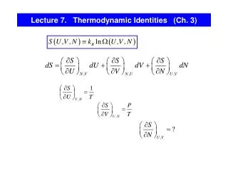
Lecture 8. Thermodynamic Identities (Ch. 3)

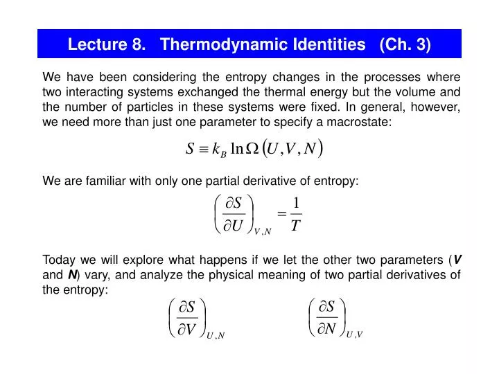
1. Lecture 8. Thermodynamic Identities (Ch. 3) We have been considering the entropy changes in the processes where two interacting systems exchanged the thermal energy but the volume and the number of particles in these systems were fixed. In general, however, we need more than just one parameter to specify a macrostate: We are familiar with only one partial derivative of entropy: Today we will explore what happens if we let the other two parameters (V and N) vary, and analyze the physical meaning of two partial derivatives of the entropy:

2. General Approach:  if monotonic as a function of U (“quadratic” degrees of freedom!), may be inverted to give When all macroscopic quantities S,V,N,U are allowed to vary: So far, we have abbreviated one of these partial derivatives: The other partial derivatives are: pressure chemical potential

3. Thermodynamic Identities - the so-called thermodynamic identity With these abbreviations:  shows how much the system’s energy changes when one particle is added to the system at fixed S and V. The chemical potential units – J.  is an intensive variable, independent of the size of the system (like P, T, density). Extensive variables (U, N, S,V...) have a magnitude proportional to the size of the system. If two identical systems are combined into one, each extensive variable is doubled in value. The thermodynamic identity holds for the quasi-static processes (T, P,  are well-define throughout the system) The 1st Law for quasi-static processes (N = const): This identity holds for small changes Sprovided T and P are well defined. The coefficients may be identified as:

4. Quasi-static Adiabatic Processes Let’s compare two forms of the 1st Law : (quasi-static processes, N is fixed, and P is uniform throughout the system) (holds for all processes) Thus, for quasi-static processes :  isentropic processes Quasistatic adiabatic (Q = 0) processes: In this case, reduces to - the change in internal energy is due to a “purely mechanical” compression (or expansion) that involves no change in entropy. (No entropy change = no heat flow).

5. 2 P S =const along the isentropic line 2* 1 Vf Vi V Caution: for non-quasistatic adiabatic processes, S might be non-zero!!! An example of a non-quasistatic adiabatic process Pr. 3.32.A non-quasistatic compression. A cylinder with air (V = 10-3 m3, T = 300K, P =105 Pa) is compressed (very fast, non-quasistatic) by a piston (S = 0.01 m2, F = 2000N, x = 10-3m). Calculate W, Q, U, and S. holds for all processes, energy conservation quasistatic, T and P are well-defined for any intermediate state quasistatic adiabatic  isentropic Q = 0 for both non-quasistatic adiabatic The non-quasistatic process results in a higher T and a greater entropy of the final state.

6. Direct approach: adiabatic quasistatic  isentropic adiabatic non-quasistatic

7. 2 To calculate S, we can consider any quasistatic process that would bring the gas into the final state (S is a state function). For example, along the red line that coincides with the adiabata and then shoots straight up. Let’s neglect small variations of T along this path ( U << U, so it won’t be a big mistake to assume T const): P U = Q = 1J 1 Vf Vi V The entropy is created because it is an irreversible, non-quasistatic compression. 2 P For any quasi-static path from 1 to 2, we must have the same S. Let’s take another path – along the isotherm and then straight up: U = Q = 2J isotherm: 1 Vf Vi V “straight up”: Total gain of entropy:

8. The inverse process, sudden expansion of an ideal gas (2 – 3) also generates entropy (adiabatic but not quasistatic). Neither heat nor work is transferred: W = Q = 0 (we assume the whole process occurs rapidly enough so that no heat flows in through the walls). 2 P Because U is unchanged, T of the ideal gas is unchanged. The final state is identical with the state that results from a reversible isothermal expansion with the gas in thermal equilibrium with a reservoir. The work done on the gas in the reversible expansion from volume Vf to Vi: 3 1 Vf Vi V The work done on the gas is negative, the gas does positive work on the piston in an amount equal to the heat transfer into the system Thus, by going 1  2  3 , we will increase the gas entropy by

9. Comment on State Functions is an exact differential (S is a state function). Thus, the factor 1/T converts Q into an exact differential. U, S and V are the state functions, Q and W are not. Specifying an initial and final states of a system does not fix the values of Q and W, we need to know the whole process (the intermediate states). In math terms, Q and W are not exact differentials and we need to use  instead of d for their increments. Analogy: in classical mechanics, if a force is not conservative (e.g., friction), the initial and final positions do not determine the work, the entire path must be specified. z(x1,y1) y - it is an exact differential if it is the difference between the values of some (state) function z(x,y) at these points: z(x2,y2) x A necessary and sufficient condition for this: If this condition holds: - cross derivatives are not equal e.g., for an ideal gas:

10. Entropy Change for Different Processes The partial derivatives of S play very important roles because they determine how much the entropy is affected when U, V and N change: The last column provides the connection between statistical physics and thermodynamics.

11. To discuss the physical meaning of these partial derivatives of S, let’s consider an ideal gas isolated from the environment, and consider two sub-systems, A and B, separated by a membrane, which, initially, is insulating, impermeable for gas molecules, and fixed at a certain position. Thus, the sub-systems are isolated from each other. (We have already considered such a system when we discussed T, but we want to proceed with P and ) Temperature UA, VA, NA UB, VB, NB Assume that the membrane becomes thermally conducting (allow exchange U while V and N remain fixed). The system will evolve to the state of equilibrium that is characterized by a maximum entropy. One of the sub-systems can increase its energy only at the expense of the other sub-system, and it’s crucial that the sub-system receiving energy increases its entropy more than the donor loses. Thus, the sub-system with a larger S/U should receive energy, and this process will continue until SA/UA and SB/UB become the same: This was our logic when we defined the stat. phys. temperature as: - the energy should flow from higher T to lower T; in thermal equilibrium, TA and TB should be the same.

12. UA, VA, NA UB, VB, NB S AB S A S B VA VAeq Let’s now fix UA,NA and UB,NB , but allow V to vary (the membrane is insulating, impermeable for gas molecules, but its position is not fixed). Following the same logic, spontaneous “exchange of volume” between sub-systems will drive the system towards mechanical equilibrium (the membrane at rest). The equilibrium macropartition should have the largest (by far) multiplicity  (U, V) and entropy S (U, V). Mechanical Equilibrium and Pressure - the sub-system with a smaller volume-per-molecule (larger P at the same T) will have a larger S/V, it will expand at the expense of the other sub-system. In mechanical equilibrium: - the volume-per-molecule should be the same for both sub-systems, or, if T is the same, P must be the same on both sides of the membrane. The stat. phys. definition of pressure:

13. The Equation(s) of State for an Ideal Gas Ideal gas: (fN degrees of freedom) The “energy” equation of state (U  T): The “pressure” equation of state (P  T): - we have finally derived the equation of state of an ideal gas from first principles! In other words, we can calculate the thermodynamic information for an isolated system by counting all the accessible microstates as a function of N, V, and U.

14. (all the processes are quasi-static) Problem: (a) Calculate the entropy increase of an ideal gas in an isothermal process. (b) Calculate the entropy increase of an ideal gas in an isochoric process. (c) What is the process in which the entropy remains constant? You should be able to do this using (a) Sackur-Tetrode eq. and (b) (a) (b) (c) a quasistatic adiabatic process = an isentropic process an adiabatic process

15. S NA UA Let’s fix VA and VB (the membrane’s position is fixed),but assume that the membrane becomes permeable for gas molecules (exchange of both U and N between the sub-systems, the molecules in A and B are the same ). Diffusive Equilibrium and Chemical Potential For sub-systems in diffusive equilibrium: UA, VA, SA UB, VB, SB In equilibrium, - the chemical potential Sign “-”: out of equilibrium, the system with the larger S/N will get more particles. In other words, particles will flow from from a high /T to a low /T.

16. Chemical Potential: examples Einstein solid: consider a small one, with N = 3 and q = 3. let’s add one more oscillator: To keep dS = 0, we need to decrease the energy, by subtracting one energy quantum.  Thus, for this system Monatomic ideal gas: At normal T and P, ln(...) > 0, and  < 0 (e.g., for He,  ~ - 5·10-20 J ~ - 0.3 eV. Sign “-”: usually, by adding particles to the system, we increase its entropy. To keep dS = 0, we need to subtract some energy, thus U is negative.

17. The Quantum Concentration  n=N/V – the concentration of molecules 0 when n increases The chemical potential increases with the density of the gas or with its pressure. Thus, the molecules will flow from regions of high density to regions of lower density or from regions of high pressure to those of low pressure .  when n nQ,   0 - the so-called quantum concentration (one particle per cube of side equal to the thermal de Broglie wavelength). When nQ >> n, the gas is in the classical regime. At T=300K, P=105 Pa , n << nQ. When n nQ, the quantum statistics comes into play.

18. Ideal Gas in a Gravitational Field Pr. 3.37. Consider a monatomic ideal gas at a height z above sea level, so each molecule has potential energy mgz in addition to its kinetic energy. Assuming that the atmosphere is isothermal (not quite right), find  and re-derive the barometric equation. note that the U that appears in the Sackur-Tetrode equation represents only the kinetic energy In equilibrium, the two chemical potentials must be equal:

19. S and CP - this is a useful result that removes the restriction of constant volume. For P = const processes, Q = CPdT  Pr. 3.29. Sketch a graph of the entropy of H20 as a function of T at P = const. S  At T0, the graph goes to 0 with zero slope. After initial fast increase of the slope, the rate of the S increase slows down (CP – almost const). When solid melts, there is a large S at T = const, another jump – at liquid–gas phase transformation. “Curving down” in both liquid and gas phases – because CP  const. water ice vapor T

20. Future Directions Although the microcanonical ensemble is conceptually simple, it is not the most practical ensemble. The major problem is that we must specify U - isolated systems are very difficult to realize experimentally, and T rather than U is a more natural independent variable.