Download
1 / 14
170 likes | 732 Vues
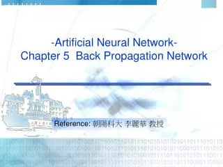
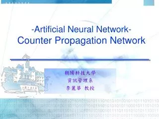
-Artificial Neural Network- Counter Propagation Network. 朝陽科技大學 資訊管理系 李麗華 教授. X 1 X 2 ‧ ‧ X n. Y 1. ‧ ‧ ‧. ‧ ‧ ‧. Y m. Introduction (1/4). Counter Propagation Network(CPN)

E N D
-Artificial Neural Network-Counter Propagation Network 朝陽科技大學 資訊管理系 李麗華 教授
X1 X2 ‧ ‧ Xn Y1 ‧ ‧ ‧ ‧ ‧ ‧ Ym Introduction (1/4) • Counter Propagation Network(CPN) - Defined by Robert Hecht-Nielsen in 1986, CPN is a network that learns a bidirectional mapping in hyper-dimensional space. - CPN learns both forward mapping (from n-space to m-space)and, if it exists, the inverse mapping (from m-space to n-space) for a set of pattern vectors.
Introduction (2/4) -Counter Propagation Network (CPN) is a an unsupervised winner-take-all competitive learning network. -The learning process consists 2 phases: The kohonen learning (unsupervised) phase & the Grossberg learning(supervised) phase.
H1 wih X1 X2 ‧ ‧ ‧ ‧ Xn whj H2 ‧ ‧ ‧ ‧ ‧ ‧ Hh Kohonen Learning Grossberg Learning Introduction (3/4) - The Architecture: Y1 Ym
Introduction (4/4) Input layer : X=[X1, X2, …….Xn] Hidden layer: also called Cluster layer, H=[H1, H2, …….Hn] Output layer: Y=[Y1, Y2, ……Ym] Weights : From InputHidden: Wih , From HiddenOutput : Whj Transfer function: uses linear type f(netj)=netj
The learning Process(1/2) The learning Process: Phase I: (Kohonen unsupervised learning) (1)Computes the Euclidean distance between input vector & the weights of each hidden node. (2)Find the winner node with the shortest distance. (3)Adjust the weights that connected to the winner node in hidden layer with △Wih* = η1(Xi - Wih* ) Phase II: (Grossberg supervised learning) • Some as (1)& (2)of phase I • Let the link connected to the winner node to output node is set as 1 and the other are set to 0. • Adjust the weights using △Wij= η2‧δ‧Hh
The learning Process(2/2) The recall process: • Set up the network • Read the trained weights. • Input the test vector, X. • Computes the Euclidean distance & finds the winner where the winner hidden node output 1 and the other output 0. • Compute the weighted sum for output nodes to derive the prediction (mapping output).
ì h=h * 1 5. Hh = í if 0 otherwise î The computation of CPN (1/4) Phase I:(Kohonen unsupervised learning) • Set up the network. • Randomly assign weights, Wih • Input training vector, X=[X1, X2, …….Xn] • Compute the Euclidean Distance to find the winner node, H* or
The computation of CPN (2/4) 6. Update weights △Wih* = η1(X1-Wih*) Wih* = Wih* + △Wih*. 7. Repeats 3 ~ 6 until the error value is small & stable or the number of training cycle is reached.
The computation of CPN (3/4) • Phase II:(Grossberg supervised learning) • Input training vector • Computes 4 & 5 of Phase I net j= ΣWhj‧ Hh Yj= net j
The computation of CPN (3/4) 3. Computes error :δj= (T j - Yj) 4. Updates weights:△W *hj= η2‧δj‧H h* W h*j= Wh* j + △Wh* j 5. Repeats 1 to 4 of Phase II until the error is very small & stable or the number of training cycle is reached.
ì h=h * 1 Hh = í if 0 otherwise î The recall computation • Set up the network. • Read the trained weights, Wih • Input testing vector (pattern), X=[X1, X2, …….Xn] • Compute the Euclidean Distance to find the winner node, H* • net j = ΣWhj‧ Hh Yj= net j
Y1 X1 Ym X2 H1 H2 0.5 H3 0.5 -0.5 -0.5 H4 The example of CPN (1/2) • Ex:Use CPN to solve XOR problem Randomly set up the weights of Wih & Whj
The example of CPN (2/2) Sol: 以下僅介紹如何計算Phase I (Phase II 計算上課說明) (1) 代入X=[-1,-1] T=[0,1] net1 =[-1-(-0.5)]2 + [-1-(-0.5)]2 = (-0.52) + (-0.52) = 0.5 net2 =[-1-(-0.5)]2 + [ 1-(-0.5)]2 = (-0.52) + ( 1.52) = 2.5 net3 = 2.5 net4 = 4.5 ∴ net 1 has minimum distance and the winner is h* = 1 (2) Update weights of Wih* △W11 = (0.5) [-1-(-0.5)] = -0.25 △W21 = (0.5) [-1-(-0.5)] = -0.25 ∴ W11 = △W11 +W11= -0.75, W21 = △W21 +W21= -0.75