Download
1 / 13
130 likes | 321 Vues
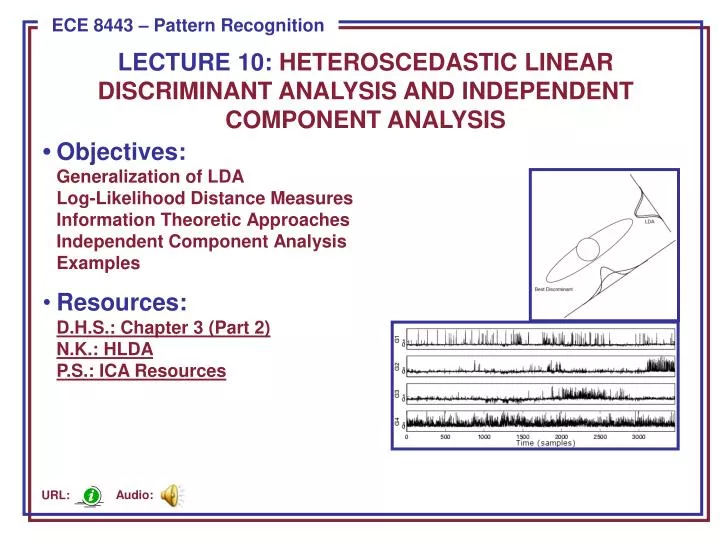
LECTURE 10: Heteroscedastic Linear Discriminant Analysis and Independent Component Analysis. • Objectives: Generalization of LDA Log-Likelihood Distance Measures Information Theoretic Approaches Independent Component Analysis Examples

E N D
LECTURE 10: Heteroscedastic Linear Discriminant Analysis and Independent Component Analysis • Objectives:Generalization of LDALog-Likelihood Distance MeasuresInformation Theoretic ApproachesIndependent Component AnalysisExamples • Resources:D.H.S.: Chapter 3 (Part 2)N.K.: HLDAP.S.: ICA Resources Audio: URL:
Linear Discriminant Analysis (Review) • Linear Discriminant Analysis (LDA) seeks to find the transformation: • that maximizes separation between the classes. This is done by maximizing a ratio of the between-class scatter and the within-class scatter: • The solution to this maximization is found by performing an eigenvalue analysis: • which produces a matrix, W, that is of dimension (c-1) rows x d columns. • Recall, however, that there was an implicit assumption of “equal covariances” – all classes had the same covariance structure: • Is there an approach that frees us from this constraint? At what cost?
Heteroscedastic Linear Discriminant Analysis (HLDA) • Heteroscedastic: when random variables have different variances. • When might we observe heteroscedasticity? • Suppose 100 students enroll in a typing class — some of which have typing experience and some of which do not. • After the first class there would be a great deal of dispersion in the number of typing mistakes. • After the final class the dispersion would be smaller. • The error variance is non-constant — it decreases as time increases. • An example is shown to the right. The two classeshave nearly the same mean, but different variances,and the variances differ in one direction. • LDA would project these classes onto a linethat does not achieve maximal separation. • HLDA seeks a transform that will account for theunequal variances. • HLDA is typically useful when classes have significant overlap.
Partitioning Our Parameter Vector • Let W be partitioned into the first p columns corresponding to the dimensions we retain, and the remaining d-p columns corresponding to the dimensions we discard. • Then the dimensionality reduction problem can be viewed in two steps: • A non-singular transform is applied to x to transform the features, and • A dimensionality reduction is performed where reduce the output of this linear transformation, y, to a reduced dimension vector, yp. • Let us partition the mean and variances as follows: • where is common to all terms and are different for each class.
Density and Likelihood Functions • The density function of a data point under the model, assuming a Gaussian model (as we did with PCA and LDA), is given by: • where is an indicator function for the class assignment for each data point. (This simply represents the density function for the transformed data.) • The log likelihood function is given by: • Differentiating the likelihood with respect to the unknown means and variances gives:
Optimal Solution • Substituting the optimal values into the likelihood equation, and then maximizing with respect to gives: • These equations do not have a closed-form solution. For the general case, we must solve them iteratively using a gradient descent algorithm and a two-step process in which we estimate means and variances from and then estimate the optimal value of from the means and variances. • Simplifications exist for diagonal and equal covariances, but the benefits of the algorithm seem to diminish in these cases. • To classify data, one must compute the log-likelihood distance from each class and then assign the class based on the maximum likelihood. • Let’s work some examples (class-dependent PCA, LDA and HLDA). • HLDA training is significantly more expensive than PCA or LDA, but classification is of the same complexity as PCA and LDA because this is still essentially a linear transformation plus a Mahalanobis distance computation.
Independent Component Analysis (ICA) • Goal is to discover underlying structure in a signal. • Originally gained popularity for applications in blind source separation (BSS), the process of extracting one or more unknown signals from noise(e.g., cocktail party effect). • Most often applied to time series analysis though it can also be used for traditional pattern recognition problems. • Define a signal as a sum of statistically independent signals: • If we can estimate A, then we can compute s by inverting A: • This is the basic principle of blind deconvolution or BSS. • The unique aspect of ICA is that it attempts to model x as a sum of statistically independent non-Gaussian signals. Why?
Objective Function • Unlike mean square error approaches, ICA attempts to optimize the parameters of the model based on a variety of information theoretic measures: • Mutual information: • Negentropy: • Maximum likelihood: • Mutual information and Negentropy are related by: • It is common in ICA to zero mean and prewhiten the data (using PCA) so that the technique can focus on the non-Gaussian aspects of the data. Since these are linear operations, they do not impact the non-Gaussian aspects of the model. • There are no closed form solutions for the problem described above, and a gradient descent approach must be used to find the model parameters. We will need to develop more powerful mathematics to do this (e.g., the Expectation Maximization algorithm).
FastICA • One very popular algorithm for ICA is based on finding a projection of x that maximizes non-Gaussianity. • Define an approximation to Negentropy: • Use an iterative equation solver to find the weight vector, w: • Choose an initial random guess for w. • Compute: • Let: • If the direction of w changes, iterate. • Later in the course we will see many iterative algorithms of this form, and formally derive their properties. • FastICA is very similar to a gradient descent solution of the maximum likelihood equations. • ICA has been successfully applied to a wide variety of BSS problems including audio, EEG, and financial data.
Summary • Introduced alternatives to PCA and LDA: • Heteroscedastic LDA: LDA for classes with unequal covariances • Introduced alternatives to mean square error approaches: • Independent Component Analysis: probabilistic approaches that attempt to uncover hidden structure or deal with non-Gaussian data • Many other forms of PCA-like algorithms exist that are based on kernels (kPCA). See Risk Minimization for more details. • Introduced the Expectation Maximization (EM) algorithm.