Download
1 / 22
250 likes | 492 Vues
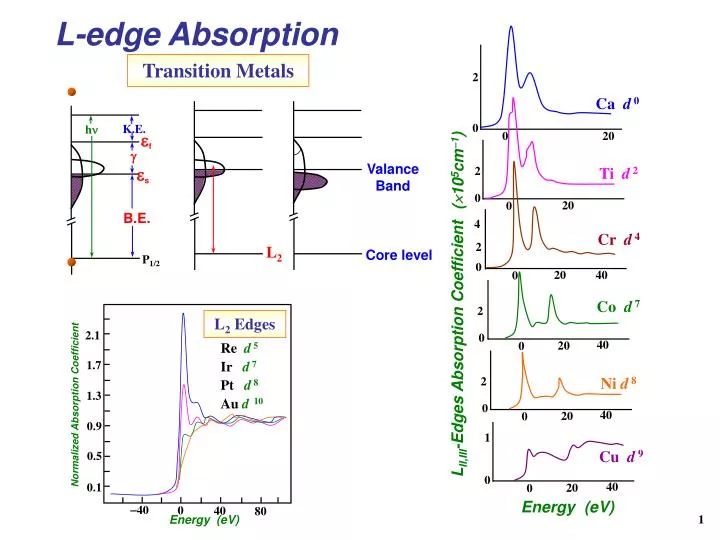
2. Ca d 0. 0. 0. 20. Valance Band. ( 10 5 cm 1 ). 2. Ti d 2. 0. 20. 0. L II,III -Edges Absorption Coefficient. 4. Cr d 4. L 2. Core level. 2. 0. 20. 40. 0. Co d 7. 2. 0. 40. 20. 0. Ni d 8. 2. 0. 40. 20. 0. 1. Cu d 9. 0. 40. 20. 0.

E N D
2 Ca d 0 0 0 20 Valance Band (105cm1) 2 Ti d 2 0 20 0 LII,III-Edges Absorption Coefficient 4 Cr d 4 L2 Core level 2 0 20 40 0 Co d 7 2 0 40 20 0 Ni d 8 2 0 40 20 0 1 Cu d 9 0 40 20 0 Energy (eV) L-edge Absorption Transition Metals K.E. h f s B.E. P1/2 Normalized Absorption Coefficient L2 Edges 2.1 Re d5 Ir d7 Pt d8 Au d10 1.7 1.3 0.9 0.5 0.1 40 0 40 80 Energy (eV)
2S+1LJ 2S+1L Dq Coulomb integral Exchange integral 2p X-ray Absorption Spectra of Transition Metal Compounds (L-Edge Absorption ) Hamiltonian of A Many Electron Atom
(a) Without considering CF: LS coupling > 2S1LJ JJ coupling < J Strong field > (b) Considering CF: < Weak field
X-ray absorption cross section: E:Photon Energy X:The perturbation acting on the system Dipole allowed transition:p d ; s p ; d f 以2p 3d為例: 3d(E) is the unoccupied 3d-projected density of state
In the atomic approach, the 2p XAS cross section for 3dn transition metal ions: (2p63dn2p53dn+1) G(3dn)is the ground state of the 3dn multiplet The important correlation effects are : (1) multiplet (2) charge transfer satellites
1F J 1D 1P 4 3F 3 3D 2 3P 1 0 Intermediate LS For Ti4 : 2p6d0 2p5d1 2P 2D 1P1 1D2 1F3 3P0,1,2 3D1,2,3 3F2,3,4 1S A1 Figure: LS jj transition for 2p53d1. In LS-coupling only the 1P1-state can be reached, but in intermediate coupling there is admixture of the 1P1-state with the 3P1-state and the 3D1-state For dipole transition (x,y,z) in Oh T1u 只有T1與T1作用,可產生A1的term。 含有T1為J = 1 , 3 , 4 J = 1 1P1 , 3P1 , 3D1 J = 3 1F3 , 3D3 , 3F3 J = 4 3F4 In Oh: J = 0 A1 1 T1 2 ET2 3 A2T1T2 4 A1ET1T2
7.0 6.0 5.0 (101) 4.0 Intensity 3.0 2.0 1.0 0.0 5 6 7 1 2 3 4 462 466 468 472 474 470 464 Energy (eV) Ti4 (d0) ☆ 10Dq 1.5
Ti3 Trivalent Td Tetrahedral D3d Trigonal Tetragonal D4h Oh Octahedral 452 462 Energy (eV) Effect on Symmetry SrTiO3 Ti4: 2p6 2p53d1 10Dq = 2.1 eV (Oh and Td ) Ti3: 2p53d1 2p53d2 Figure: Crystal field multiplet calculations. In all spectra the cubic crystal field strength (10Dq) is 2.1 eV. From bottom to top : a calculation in octahedral symmetry, tetragonal (D4h) symmetry, trigonal (D3d) symmetry, tetrahedral symmetry (10Dq = 2.1eV) and a calculation for Ti3 (3d1 2p53d2).
0eV 0.3eV 0.6eV 0.9eV (101) (101) (101) (101) (101) Intensity Intensity Intensity Intensity Intensity Energy (eV) Energy (eV) Energy (eV) Energy (eV) Energy (eV) 1.5eV 1.2eV 1.8eV 2.1eV (101) (101) (101) Intensity Intensity Intensity 3.3eV 2.4eV 2.7eV 3.0eV (101) (101) (101) (101) Energy (eV) Energy (eV) Energy (eV) Intensity Intensity Intensity Intensity Energy (eV) Energy (eV) Energy (eV) 3.9eV Energy (eV) 3.6eV 4.2eV 4.5eV (101) (101) (101) (101) Intensity Intensity Intensity Intensity Energy (eV) Energy (eV) Energy (eV) Energy (eV) Effect onDq Ti4 (d0) 2p6d0 → 2p5d1
Effect on the crystal field strength (Dq) V3 in Oh Mn2 MnF2 Intensity ☆10Dq 0.75 eV 24 Intensity 21 650 660 Energy (eV) Exp 18 Mn2 in Oh Intensity Cal 15 638 648 Energy (eV) 18 12 VF3 15 09 Intensity 12 06 ☆10Dq 1.5 eV Intensity 09 03 Exp 06 00 Cal 520 510 530 03 Energy (eV) 518 528 Energy (eV) 00 655 635 645 Energy (eV) Dq(eV) Dq(eV)
Fe2 in Oh Absorbance Experiment 18 Calculation 700 705 710 715 720 730 725 15 Energy (eV) 12 Intensity 09 Absorbance 06 03 B C A Experiment Calculation 00 700 705 710 715 720 725 730 Energy (eV) 705 715 725 Energy (eV) Dq(eV) Figure: Comparison between experimental and calculated (3d6 to 2p53d7 multiplet ) L2,3 edge spectra for the high-spin Fe(phen)2(NCS)2 isomer. Calculation is made considering Oh symmetry with a 10Dq cubic crystal field parameter equal to 0.5eV. Figure: Comparison between experimental and calculated (3d6 to 2p53d7 multiplet ) L2,3 edge spectra for the low-spin Fe(phen)2(NCS)2 isomer. Calculation is made considering Oh symmetry with a 10Dq cubic crystal field parameter equal to 2.2eV.
0.3eV 0.6eV 0.9eV 0eV 1.5eV 1.2eV (101) (101) (101) (101) (101) (101) Intensity Intensity Intensity Intensity Intensity Intensity Energy (eV) Energy (eV) Energy (eV) Energy (eV) Energy (eV) Energy (eV) 2.1eV 1.8eV (101) (101) Intensity Intensity Energy (eV) Energy (eV) 3.3eV 2.7eV 3.0eV 2.4eV (101) (101) (101) (101) Intensity Intensity Intensity Intensity 4.5eV 4.2eV 3.9eV 3.6eV (101) (101) (101) (101) Intensity Intensity Intensity Intensity Energy (eV) Energy (eV) Energy (eV) Energy (eV) Energy (eV) Energy (eV) Energy (eV) Energy (eV) Fe2 (d6) 2p6d6 → 2p5d7
2p6dn 2p5dn1 2p6dn1Lm1 2p5dnLm1 2p6dn 2p5dn1 2p6dn1Lm1 2p5dn2Lm1 Multiplet with Charge transfer For 3d-TM 2p63dn 2p53dn1 <A> (2p63dn) (2p63dn1) (2p53dn1) (2p53dn) <B> (2p63dn) (2p63dn1) (2p53dn1) (2p53dn2) Charge transfer <A> MLCT <B> LMCT
2.0 2.0 Intensity (101) Intensity (101) 1.0 1.0 0.0 0.0 728 721 707 714 735 742 728 721 707 714 735 742 Energy (eV) Energy (eV) Fe2+ in Low Spin , Dq=2.2eV with CT Fe2+ in High Spin , Dq=0.9eV with CT
LIII HS Arbitrary Scale LII HS-1, 298K HS-1, multiplet calculated with charge transfer HS-1, multiplet calculated without charge transfer LS LS-1, 15K LS-1, multiplet calculated with charge transfer LS-1, multiplet calculated without charge transfer 695 715 700 705 735 725 730 710 720 Photon Energy (eV) Multiplet Calculation HS:10Dq 0.91eV LS:10Dq 2.13eV Experimental and Calculated LII,III-absorption edge of Fe(phen)2(NCS)2 on 298K, 15K JACS 2000, 122,5742-7
Co Intensity LiCoO2 3 Li0.2Co0.8O Li0.2Co0.9O Mn CoO 2 Li2MnO3 770 780 795 775 790 785 Intensity 4 LiMn2O4 Energy (eV) 3.5 LiMnO2 3 MnO 2 632 647 642 652 637 Energy (eV) L2,3 absorption of TM with various oxidation states Figure: The Co L2,3 x-ray absorption spectra of CoO、Li0.2Co0.9O、Li0.2Co0.8O and LiCoO2. Figure: The Mn L2,3 x-ray absorption spectra of MnO、LiMnO2、LiMn2O4 and Li2MnO3.
[Sr] [Sr] Normalized Intensity 1.0 1.0 Normalized Intensity 0.9 0.7 0.8 0.5 0.5 0.3 0.4 0.1 0.2 0.0 0.0 700 710 720 730 Photon Energy (eV) 450 460 465 470 455 Photon Energy (eV) La1-xSrxFeO3 Fe L2,3 XAS La1-xSrxTiO3 Ti L2,3 XAS SrTiO3 SrFeO3 LaFeO3 LaTiO3 Figure: The 2p x-ray absorption spectra of the La1-xSrxTiO3-system. The solids lines are the results of crystal field multiplet calculations: At the bottom the 3d1 [2T2] 2p53d2 transition is given and the solid line simulating the SrTiO3 spectrum relates to the 3d0 [1A1] 2p53d1 Figure: The 2p x-ray absorption spectra of the La1-xSrxFeO3 system.
O K-edge MnO2 Sc2O3 Normalized Intensity Fe2O3 TiO2 Ti2O3 Fe3O4 Normalized Intensity VO2 NiO V2O3 CuO Cr2O3 540 530 550 Energy (eV) 540 530 550 Energy (eV) (b) (a) Figure: (a) and (b) Oxygen 1s x-ray-absorption spectra : the shaded area is assigned to oxygen p character in the transition metal 3d band . The broader structure above is assigned to oxygen p character in the metal 4s and 4p bands . The vanadium edges are distorted by the tail of the vanadium L2 edge.
(a) L2,3 Photoabsorption of Nickel Absorption Intensity 120 Continuum State 1/2 1/2 80 Core State 40 3/2 1/2 3/2 L2 A’ L3 A 1/2 Building Energy 3/2 850 890 870 Photon Energy (eV) 1/2 (b) Magnetic Circular Dichroism Intensity Difference 1/2 4 1/2 j mj B L3 m 1 m 1 L R 0 L-R L2 B’ 4 8 850 890 870 Photon Energy (eV) Magnetic Circular Dichroism (MCD) mj 1 Figure: Dipole transition from a core p level to a continuum s state with left and right circularly polarized light, and the resulting circular dichioism in the photoemission .
0.05 0.8 Co LIII (Co40/Cr5)20/Mo/MgO Intensity 0.6 0.00 Co LII 0.4 0.2 0.05 780 760 800 820 Photon Energy (eV) 810 820 800 760 770 790 780 Photon Energy (eV) (b) (a) Figure (a): A normalized soft-x-ray absorption spectrum of sample (Co40Å/ Cr5Å)10/ Mo/MgO(100) under different magnetized directions . Figure (b): The net difference of the spectrum in Fig. (a) , which is the MCD intensity .
0.6 IRON 0.8 0.4 0.4 0.2 0.0 0.0 700 740 700 720 760 740 720 760 4S1/2 3d3/2 3d5/2 1/2 1/2 1/2 3/2 3/2 1/2 3/2 5/2 1/2 1/2 3/2 5/2 1/2 1/2 1/2 3/2 1/2 3/2 2P1/2 2P3/2 Photon Energy (eV) Left circularly polarized light:mj 1 Right circularly polarized light:mj 1 1. C.T. Chen, Y.U. Idzerda,H.-J. Lin, N.V. Smith, G. Meigs, E. Chaban, G. H. Ho, E. Pellegrin, Sette, Phys Rev. Lett. 75, 152(1994). 2. H. Ebert, G. Schutz, Spin-Orbit Influenced Spectroscopies of magnetic Solids, 1996, p161.
(a) Transmission 1.2 L2 L3 1.0 I I 0.8 Is (b) 0.6 IRON Absorption 0.4 0.2 0.0 0.1 0.2 MCD Integration (c) MCD 0.0 0.0 q 0.2 0.1 p 0.4 0.2 0.6 XAS Integration (d) XAS 0.8 4.0 r 0.4 2.0 0.0 0.0 760 720 740 700 Photon Energy (eV) Figure : L2,3-edge XAS and MCD spectrum of iron: (a) Transmission spectra of Fe/parylene thin films, and of the parylene substrates alone, taken at two opposite saturation magnetizations. (b) The XAS absorption spectra calculated from the transmission data shows in (a). (c) and (d) are the MCD and summed XAS spectra and their integrations calculated from the spectra shown in (b). The dotted line shown in (d) is the two-step like function for edge-jump removal before the integration. The p and q shown in (c) and the r shown in (d) are the three integrals needed in the sum-rule analysis. XMCD Reference: Coord. Chem. Rev. 249(2005) 3-30