Download
1 / 19
200 likes | 538 Vues
Exp. 20 - video (time: 41:13 minutes). Exp. 20: Spectrophotometric Analysis: Determination of the Equilibrium Constant for a Reaction. Chemical Equilibrium. Previously we have assumed that chemical reactions results in complete conversion of reactants to products:

E N D
Exp. 20 - video (time: 41:13 minutes) Exp. 20: Spectrophotometric Analysis: Determination of the Equilibrium Constant for a Reaction
Chemical Equilibrium Previously we have assumed that chemical reactions results in complete conversion of reactants to products: A + B C + D No A or B remaining or possibly an excess of A or B but not both and eventually reaction stops. Many chemical reactions do not completely convert reactants to products. Stop somewhere between no rxn and complete rxn. A + B C + D some left some formed reversible (both directions) A + B C + D A + B C + D exchange, constant conc., Ratef = Rater “equilibrium”
Chemical Equilibrium • Therefore, many reactions do not go to completion but rather form a mixture of products and unreacted reactants, in a dynamic equilibrium. • A dynamic equilibrium consists of a forward reaction, in which substances react to give products, and a reverse reaction, in which products react to give the original reactants. • Chemical equilibrium is the state reached by a reaction mixture when the rates of the forward and reverse reactions have become equal.
Graphically we can represent this A + B C + D The concentrations and reaction rate (less collisions, less component) of A and B decreases over time as the concentrations and reaction rate of C and D increases (more collisions, more component) over time until the rates are equal and the concentrations of each components reaches a constant. This occurs at what we call equilibrium -- Rf = Rr. If the rates are equal, then there must be a relationship to show this.
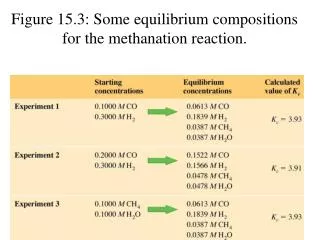
3H2 + CO CH4 + H2O Rf=Rr 3H2 + CO CH4 + H2O rate decreases over time CH4 + H2O 3H2 + CO rate increases over time Ebbing, D. D.; Gammon, S. D. General Chemistry, 8th ed., Houghton Mifflin, New York, NY, 2005.
If we assume these reactions are elementary rxns (based on collisions), we can write the rate laws directly from the reaction: A + B C + D Rf = kf [A][B] For the reverse reaction we have, C + D A + B Rr = kr [C][D] We know at equil that Rf = Rr ;therefore, we can set these two expressions as equal kf [A][B] = kr [C][D] Rearrange to put constants on one side we get
Constant divided by constant just call a new constant K. This ratio is given a special name and symbol called equilibrium constant K relating to the equilibrium condition at a certain temperature (temp dependent) for a particular reaction relating conc of each component. This is basically a comparison between forward and reverse reaction rates. At equilibrium, the ratio of conc of species must satisfy K.
The Equilibrium Constant • Every reversible system has its own “position of equilibrium”- K- under any given set of conditions. • The ratio of products produced to unreacted reactants for any given reversible reaction remains constant under constant conditions of pressure and temperature. If the system is disturbed, the system will shift and all the concentrations of the components will change until equilibrium is re-established which occurs when the ratio of the new concentrations equals "K". Different constant conc but ratio same as before. • The numerical value of this ratio is called the equilibrium constant for the given reaction, K.
The Equilibrium Constant • The equilibrium-constant expression for a reaction is obtained by multiplying the equil concentrations ( or partial pressures) of products, dividing by the equil concentrations (or partial pressures) of reactants, and raising each concentration to a power equal to its coefficient in the balanced chemical equation. c • The molar concentration of a substance is denoted by writing its formula in square brackets for aq solutions. For gases can put Pa - atm. As long as use M or atm, K is unitless; liquids and solids = 1; setup same for all K’s (Ka, Kb, etc.) • Temp dependent; any changes, ratio will still equal K when equil established
Fe3+ + SCN- FeSCN2+K? In our experiment, we will determine the K for the following reaction: Fe3+ + SCN- FeSCN2+
If we can determine x, we can solve for K for this reaction. First part of experiment involves making a calibration curve for [FeSCN2+]
Calibration Curve We basically force the [FeSCN2+] to equal the initial [SCN-] by using a 1:1000 ratio of SCN- to Fe3+ pg 139: 20.00 mL of 2.00 x 10⁻⁴ M KSCN 20.00 mL of 0.200 M Fe(NO3)3 Therefore, [SCN-]o diluted within rxn = [FeSCN2+]eq for calibration only not actual K experiment
Calibration Curve [SCN-]o = [FeSCN2+]eqwithin rxn (meaning taking into account dilution) No.1 Standard (pg 139) 20.00 mL of 2.00 x 10⁻⁴ M KSCN 20.00 mL of 0.200 M Fe(NO3)3 CV = CV (2.00 x 10⁻⁴ M SCN-) (20.00 mL) = CSCN- diluted No. 1 (40.00 mL) [CSCN-diluted No.1] = 1.00 x 10⁻⁴ M = [FeSCN2+]No. 1
10.0 x 10⁻⁵ 1.00 x 10⁻⁴ 5.00 x 10⁻⁵ 2.50 x 10⁻⁵ No. 2 standard (1.00 x 10⁻⁴ M SCN-) (10.00 mL) = CSCN- diluted No. 2 (20.00 mL) [CSCN-diluted No. 2] = 5.00 x 10⁻⁵ M = [FeSCN2+]No. 2 No. 3 is done same way and then measure the absorbance at 460 nm (watch filter on spec 20) of each for calibration curve. Tip for plotting: make the three conc the same power of 10 and label axis conc x 10-5 M. blank: 0.00 M0.00
Preparation of solutions for K experiment pg 139: Fe3+ solution – CV = CV Make solutions No. 1 -3 from stock 0.200 M; skip No.4 0.100 0.0500 0.0250
Preparation of solutions for K experiment pg. 140: Initial [SCN-]o same dilution across (5 mL SCN- and 5 mL Fe3+) [SCN-]o = 1.00 x 10⁻⁴ M (skip No.4) Initial [Fe3+]o same dilution but different stock of Fe3+ (5 mL/5 mL) [Fe3+]o = ½ [Fe3+ solution pg 139] (skip No. 4) 0.100 M 0.0500 M 0.0250 M [SCN-]o 1.00 x 10⁻⁴ 1.00 x 10⁻⁴ 1.00 x 10⁻⁴ [Fe3+]o 0.0500 M 0.0250 M 0.0125 M
Determination of K • Obtain calibration curve from first three solutions (top of pg 139); this plot will allow you to determine the [FeSCN2+]eq for each of the three experimental mixtures. • Mix solutions for exp 1 (pg 140), obtain absorbance from spec 20 at 460 nm, read absorbance off calibration curve for [FeSCN2+]eq; technically the x in K expression
Determination of K • Bottom table pg 140 • [Fe3+]eq = [Fe3+]o – x = [Fe3+]o – [FeSCN2+]eq • [SCN-]eq = [SCN-]o – x = [SCN-]o – [FeSCN2+]eq • Plug values into K expression and solve for K • Repeat for exp 2 and 3 exp1 exp 2exp 3 spec 20 spec 20 spec 20 graph = “x” graph graph eq [Fe3+]o – [FeSCN2+]eq = 0.0500 – graphexp1 0.0250 – graphexp2 0.0125 – graphexp3 eq [SCN-]o – [FeSCN2+]eq = 1.00 x 10⁻⁴ – graphexp1 1.00 x 10⁻⁴ – graphexp2 1.00 x 10⁻⁴ – graphexp3 eq
Goal: Average K for reaction and std dev. Only computer plot required but make sure change axis to some small increment. Chemicals: Take only 45 mL of each component.