Download

1 / 57
580 likes | 596 Vues
CHAPTER 66 MODULATION AND DEMODULATION. LEARNING OBJECTIVES. What is a Carrier Wave? Radio Frequency Spectrum Need for Modulation Modulation Methods of Modulation Amplitude Modulation Percent Modulation Upper and Lower Sidebands Mathematical Analysis of a Modulated Carrier Wave

E N D
LEARNING OBJECTIVES • What is a Carrier Wave? • Radio Frequency Spectrum • Need for Modulation • Modulation • Methods of Modulation • Amplitude Modulation • Percent Modulation • Upper and Lower Sidebands • Mathematical Analysis of a Modulated Carrier Wave • Power Relation in an AM Wave • Forms of Amplitude Modulation
LEARNING OBJECTIVES • Generation of SSB • Methods of Amplitude Modulation • Modulating Amplifier Circuit • Frequency Modulation • Modulation Index • Deviation Ratio • Percent Modulation • FM Sidebands • Modulation Index and Number of Sidebands • Demodulation or Detection • Essentials of AM Detection • Transistor Detectors for AM Signals
LEARNING OBJECTIVES • Quadrature Detector • Frequency Conversion • Standard Superhet AM Receiver • FM Receiver • Comparison between AM and FM • The Four Fields of FM
WHAT IS A CARRIER WAVE • It is a high-frequency undamped radio wave produced by radio-frequency oscillators . As seen from Fig. 66.1, the output of these oscillators is first amplified and then passed on to an antenna. Fig. 66.1
WHAT IS A CARRIER WAVE • This antenna radiates out these high-frequency (electromagnetic) waves into space. These waves have constant amplitude and travel with the velocity of light. • They are inaudible i.e. by themselves they cannot produce any sound in the loudspeaker of a receiver. As their name shows, their job is to carry the signal (audio or video) from transmitting station to the receiving station. The resultant wave is called modulated carrier wave.
NEED FOR MODULATION • There are three main hurdles in the process of such direct transmission of audio-frequency signals: • They have relatively short range, • If everybody started transmitting these low-frequency signals directly, mutual interference will render all of them ineffective • Size of antennas required for their efficient radiation would be large i.e. about 75 km.
MODULATION • It is the process of combining an audio frequency (AF) signal with a radio frequency (RF) carrier wave. The AF signal is also called a modulating wave and the resultant wave produced is called modulated wave. Fig 66.2
METHODS OF MODULATION • The mathematical expression for a sinusoidal carrier wave is • Obviously, the waveform can be varied by any of its following three factors or parameters • — the amplitude, • — the frequency • φ — the phase
AMPLITUDE MODULATION • In this case, the amplitude of the carrier wave is varied in proportion to the instantaneous amplitude of the information signal or AF signal. Obviously, the amplitude (and hence the intensity) of the carrier wave is changed but not its frequency. • In summary • fluctuations in the amplitude of the carrier wave depend on the signal amplitude, • rate at which these fluctuations take place depends on the frequency of the audio signal.
AMPLITUDE MODULATION • The process of amplitude modulation is shown graphically in Fig. 66.3. Fig. 66.3
PERCENT MODULATION • It indicates the degree to which the AF signal modulates the carrier wave. • The ratio B/A expressed as a fraction is called modulation index (MI). • Modulation may also be defined in terms of the values referred to the modulated carrier wave
UPPER AND LOWER SIDE FREQUENCIES • An unmodulated carrier wave consists of only one single-frequency component of frequency . When it is combined with a modulating signal of frequency fm, heterodyning action takes place. As a result, two additional frequencies called side frequencies are produced. • The original carrier frequency component, . • A higher frequency component ( + ). It is called the sum component. • A lower frequency component ( – ). It is called the difference component. • The two new frequencies are called the upper-side frequency (USF) and lower-side frequency (LSF) respectively
UPPER AND LOWER SIDE FREQUENCIES • These are shown in time domain in Fig. 66.4 (a) and in frequency domain in Fig. 66.4 (b). Fig. 66.4
UPPER AND LOWER SIDEBANDS • In a broadcasting station, the modulating signal is the human voice (or music) which contains waves with a frequency range of 20-4000 Hz. Each of these waves has its own LSF and USF. When combined together, they give rise to an upper-side band (USB) and a lower-side band (LSB) as shown in Fig. 66.5. Fig. 66.5
MATHEMATICAL ANALYSIS OF A MODULATED CARRIER WAVE • The equation of an unmodulated carrier wave is • It is seen that the modulated wave contains three components
FORMS OF AMPLITUDE MODULATION • DSB-SC • It stands for double-sideband suppressed carrier system [Fig. 66.6 (a)]. Here, carrier component is suppressed thereby saving enormous amount of power. Carrier signal contains 66.7 per cent of the total transmitted power for m = 1, Hence, power saving amounts to 66.7% at 100% modulation Fig. 66.6
FORMS OF AMPLITUDE MODULATION • SSB-TC : As shown in Fig. 66.6 (b), in this case, one sideband is suppressed but the other sideband and carrier are transmitted. It is called single sideband transmitted carrier system. For m = 1, power saved is 1/6 of the total transmitted power, • SSB-SC: This is the most dramatic suppression of all because it suppresses one sideband and the carrier and transmits only the remaining sideband as shown in Fig. 66.6 (c). In the standard or double-sideband full-carrier (DSB.FC) AM, carrier conveys no information but contains maximum power.
FORMS OF AMPLITUDE MODULATION • The advantage of SSB-SC system are as follows : • Total saving of 83.3% in transmitted power (66.7% due to suppression of carrier wave and 16.6% due to suppression of one sideband). Hence, power is conserved in an SSB transmitter. • Bandwidth required is reduced by half i.e. 50%. Hence, twice as many channels can be multiplexed in a given frequency range. • The size of power supply required is very small. This fact assumes vital importance particularly in a spacecraft. • Since the SSB signal has narrower bandwidth, a narrower passband is permissible within the receiver, thereby limiting the noise pick up.
METHODS OF AMPLITUDE MODULATION • There are two methods of achieving amplitude modulation : • Amplifier modulation, • Oscillator modulation. • Block diagram of Fig. 66.7 illustrates the basic idea of amplifier modulation. Here, carrier and AF signal are fed to an amplifier and the result is an AM output . The modulation process takes place in the active device used in the amplifier. Fig. 66.7
BLOCK DIAGRAM OF AN AMTRANSMITTER • Fig. 66.8 shows the block diagram of a typical transmitter. Fig. 66.8
BLOCK DIAGRAM OF AN AMTRANSMITTER • The carrier wave is supplied by a crystal-controlled oscillator at the carrier frequency. It is followed by a tuned buffer amplifier and an RF output amplifier. • The source of AF signal is a microphone. The audio signal is amplified by a low level audio amplifier and, finally, by a power amplifier. It is then combined with the carrier to produce a modulated carrier wave which is ultimately radiated out in the free space by the transmitter antenna as shown.
FREQUENCY MODULATION OR CAD SIMULATION DIAGRAM • In this modulation, it is only the frequency of the carrier which is changed and not its amplitude. Fig. 66.9
FREQUENCY MODULATION OR CAD SIMULATION DIAGRAM • The amount of frequency deviation (or shift or variation) depends on the amplitude (loudness) of the audio signal. Louder the sound, greater the frequency deviation and vice-versa. • However, for the purposes of FM broadcasts, it has been internationally agreed to restrict maximum deviation to 75 kHz on each side of the centre frequency for sounds of maximum loudness. Sounds of lesser loudness are permitted proportionately less frequency deviation. • The rate of frequency deviation depends on the signal frequency.
MODULATION INDEX • Unlike amplitude modulation, this modulation index can be greater than unity. By knowing the value of , we can calculate the number of significant sidebands and the bandwidth of the FM signal.
DEVIATION RATIO • It is the worst-case modulation index in which maximum permitted frequency deviation and maximum permitted audio frequency are used.
PERCENT MODULATION • When applied to FM, this term has slightly different meaning than when applied to AM. In FM, it is given by the ratio of actual frequency deviation to the maximum allowed frequency deviation.
FM SIDEBANDS • If is the centre frequency and fm the frequency of the modulating signal, then carrier contains the following frequencies :
MODULATION INDEX AND NUMBER OF SIDEBANDS • It is found that the number of sidebands • depends directly on the amplitude of the modulating signal, • depends inversely on the frequency of the modulating signal. • Since frequency deviation is directly related to the amplitude of the modulating signal, the above two factors can be combined in one factor called modulation index. • The number of pairs of sidebands • increases as frequency deviation (or amplitude of modulating signal) increases. • increases as the modulating signal frequency decreases
MATHEMATICAL EXPRESSION FOR FM WAVE • The unmodulated carrier is given by • The modulating signal is given by
DEMODULATION OR DETECTION • The process of recovering AF signal from the modulated carrier wave is known as demodulation or detection. • The demodulation of an AM wave involves two operations : • rectification of the modulated wave and • elimination of the RF component of the modulated wave • Demodulation of an FM wave involves three operations • conversion of frequency changes produced by modulating signal into corresponding amplitude changes • rectification of the modulating signal and • elimination of RF component of the modulated wave
DIODE DETECTOR FOR AM SIGNALS • Diode detection is also known as envelope-detection or linear detection. In appearance, it looks like an ordinary half-wave rectifier circuit with capacitor input as shown in Fig. 66.10. Fig. 66.10
DIODE DETECTOR FOR AM SIGNALS • It is called envelope detection because it recovers the AF signal envelope from the composite signal. Similarly, diode detector is called linear detector because its output is proportional to the voltage of the input signal. • Advantages • They can handle comparatively large input signals • They can be operated as linear or power detectors • They rectify with negligible distortion and, hence, have good linearity. • They are well-adopted for use in simple automatic-gain control circuits.
DIODE DETECTOR FOR AM SIGNALS • Disadvantages • They do not have the ability to amplify the rectified signal by themselves as is done by a transistor detector . However, it is not a very serious drawback since signal amplification can be affected both before and after rectification. • While conducting, the diode consumes some power which reduces the Q of its tuned circuit as well as its gain and selectivity.
TRANSISTOR DETECTORSFOR AM SIGNALS • Transistors can be used as detector amplifiers i.e. both for rectification and amplification. As shown in Fig. 66.11, the RF signal is applied at the base-emitter junction where rectification takes place. The amplification of the recovered signal takes place in the emitter collector circuit. Fig. 66.11
FM DETECTION • A simple method of converting frequency variations into voltage variations is to make use of the principle that reactance (of coil or capacitor) varies with frequency. • When an FM signal is applied to an inductor, the current flowing through it varies in amplitude according to the changes in frequency of the applied signal. • Now, changes in frequency of the FM signal depend on the amplitude of the modulating AF signal. Hence, the current in the inductor varies as per the amplitude of the original modulating signal. In this way, frequency changes in FM signal are converted into amplitude changes in current.
QUADRATURE DETECTOR • This detector depends on the frequency/phase relationship of a tuned circuit. It uses only one tuned circuit and is becoming increasingly popular in the integrated FM strips. • Let us first consider the general principle. A sinusoidal current is given by the equation • The voltage across the inductor (assumed pure) leads the current I by 90.
FREQUENCY CONVERSION • Need • It is very difficult to design amplifiers which give uniformly high gain over a wide range of radio frequencies used in commercial broadcast stations. However, it is possible to design amplifiers which can provide high-gain uniform amplification over a narrow band of comparatively lower frequencies called intermediate frequencies (IF). • Basic Principle • The frequency conversion can be achieved by utilizing the heterodyne principle. For this purpose, the modulated RF signal is mixed (in a mixer) with an unmodulated RF signal produced by local oscillator as shown in Fig. 66.12
FREQUENCY CONVERSION Fig. 66.12
FREQUENCY CONVERSION • Heterodyning Action • Suppose the carrier signal of frequency is heterodyned with another signal of frequency , then two additional signals are produced whose frequencies are
SUPERHETRODYNE AM RECEIVER Fig 66.13
SUPERHETRODYNE AM RECEIVER • Let us assume that the incoming signal frequency is 1500 kHz. It is first amplified by the R.F. amplifier. • Next, it enters a mixer circuit which is so designed that it can conveniently combine two radio frequencies—one fed into it by the R.F. amplifier and the other by a local oscillator. • The local oscillator is an RF oscillator whose frequency of oscillation can be controlled by varying the capacitance of its capacitor. In fact, the tuning capacitor of the oscillator is ganged with the capacitor of the input circuit so that the difference in the frequency of the selected signal and oscillator frequency is always constant.
SUPERHETRODYNE AM RECEIVER • When two alternating currents of these two different frequencies are combined in the mixer transistors, then phenomenon of beats is produced. In the present case, the beat frequency is 1955-1500 = 455 kHz. Since this frequency is lower than the signal frequency but still above the range of audio frequencies, it is called intermediate frequency (IF). • The 455 kHz output of the mixer is then passed on to the IF amplifier which is fixed tuned to 455 kHz frequency. In practice, one or more stages of IF amplification may be used.
SUPERHETRODYNE AM RECEIVER • The output of IF amplifier is demodulated by a detector which provides the audio signal. • This audio signal is amplified by the audio-frequency (AF) amplifier whose output is fed to a loud-speaker which reproduces the original sound.
STANDARD SUPERHET AM RECEIVER Fig. 66.14