Download
1 / 21
210 likes | 460 Vues
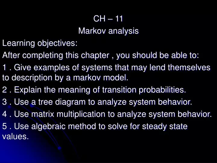
CH – 11 Markov analysis Learning objectives: After completing this chapter , you should be able to: 1 . Give examples of systems that may lend themselves to description by a markov model. 2 . Explain the meaning of transition probabilities. 3 . Use a tree diagram to analyze system behavior.

E N D
CH – 11 Markov analysis Learning objectives: After completing this chapter , you should be able to: 1 . Give examples of systems that may lend themselves to description by a markov model. 2 . Explain the meaning of transition probabilities. 3 . Use a tree diagram to analyze system behavior. 4 . Use matrix multiplication to analyze system behavior. 5 . Use algebraic method to solve for steady state values.
Summary Markov analysis can be useful for describing the behavior of a certain class of system that change from state to state on a period – by – period basis according to know transition probabilities. Customers patterns , market share , and equipment breakdowns sometimes lend themselves to description in markov terms.
Markov process: Steady state: Transition matrix: A closed system that change from state to state according to stable transition probabilities. The long- term tendencies of amarkov system to be in its various states. A matrix that shows the probabilities of markov system changing from is current state to each possible state in the next period. Glossary
CH – 11 Markov analysis A markov system has these characteristics 1 . It will operate or exist for a number of periods. 2 . In each period , the system can assume one of a number of states or conditions. 3 . System changes between states from period to period can be described by transition probabilities , which remain constant. Example of system that may be described as markov Proportion of customers Who buy brand A Brand B Brand C etc Brand switching Probability That a customer Will switch from Brand A to brand B , etc
Transition probabilities Which indicate the tendencies of the system to change from one period to the next Example : A car rent agency that has to offices at each of a city’s two airports. Customers are allowed to return a rented car to either airport , regardless of which airport they rented from. Suppose that the manager of the rented agency has made a study of return behavior and has found the following Info :
70% of cars rented from airport A tend to be returned to that airport , and 30% of A tend to returned to B. 10% of cars rented from airport B are returned to airport A. and 90% returned to B. Transition probabilities for car agency Returned to A B A .70 .30 = 1.00 rented from B .10 .90 = 1.00
The manager has several questions concerning the system : 1 . What proportion of cars will be returned to each airport at the short-run , over the next several days. 2 . What proportion of cars will be to each location over the long – run . Methods of analysis For a short – run 1. Tree diagram 2. Matrix multiplication For a long – run 3. Algebraic method.
Tree diagram For one period 0 1 A A At this point B A = .70 B = .30 0 1 A B B = .90 B A = .10 .70 Strating from .30 .10 Strating from .90
What we are doing for Several periods ?
Example :- Use the Info. In the previous example , and prepare a tree diagram for two period. Then compute joint probabilities and use them to determine how many cars will be at location A if A originally has 100 cars and location B has 80 cars . Joint probabilities Period A B 0 1 2 .70x.70=.49 .70x.30=.21 A .30x.10=.03 .30x.90=.27 A B .52 .48 A A A B .70 .70 .30 .10 .30 .90
Joint probabilities Period A B 0 1 2 .10x.70=.07 .10x.30=.03 A .90x.10=.09 .90x.90=.81 A B .16 .84 A A A B At zero point A=100 cars , B = 80 cars A B 100(.52) + 80(.16) = 64 cars in A at the second period. .70 .10 .30 .10 .90 .90
→ matrix multiplication We need two matrix to use I solution : 1 . Shares matrix 2 . Transition probabilities matrix. Share’s matrix can be obtained from the calculations period to period . But for the first period ( zero period ) we may assume the shares. for our example : shares for A , B would be this mean that all cars are in A. for period one A B = 1(.70) 1(.30) + 0(.10) +0(.90) This share will Use in the next period.
→ for the 2 period A B = .70(.70) = .49 .70(.30) = .21 .30(.10) = .03 .30(.90) = .27 .52 .48 This share will Use in the 3 period → algebraic Solution The basic Equation is A+B = 1
From the transition probability tape we can develop the equation , for A and for B A = .70A + .10B B = .30A + .90B A = .70A + .10B B = 1-A A = .70A + .10(1-A) B = 1-.25 A = .70A + .10 - .10A B = .75 A = .60A + .10 A - .60A = .10 .40A = .10 A = = .25
→ Analysis for 3x3 matrix Example :- X Y Z X .70 .20 .10 Y .40 .50 .10 Z .30 .10 .60 Tree diagram solve for 2 period stating from X.
Period 0 1 2 x x y z x x y y z x z y z Joint probabilities x share .70(.70) = .49 .20(.40) = .08 .10(.30) = .03 .60 y share .70(.20) = .14 .20(.50) = .10 .10(.10) = .01 .25 z share .70(.10) = .07 .20(.10) = .02 .10(.60) = .06 .15 The same if you want to solve starting Y or Z ?
Matrix multiplication Solution Period : starting from x x y z 1(.70) 1(.20) 1(.10) 0 0(.40) 0(.50) 0(.10). 0(.30) 0(.10) 0(.60) .70 .20 .10 2 .70 .20 .10 .70(.70) .70(.20) .70(.10) .20(.40) .20(.50) .20(.10) .10(.30) .10(.10) .10(.60) .60 .25 .15 For the 3ed period , and so on .
Algebraic solution equations 1. X = .70x + .40y + .30z Y = .20x + .50y + .10z Z = .10x + .10y + .60z 1 = x + y +z basic equation 2. Eliminate one the equations , but not the basic equation. Suppose the third equation is eliminated . Z = 1 – X - Y
3. Substitute for Z in the first and second equations X = .70x + .40y + .30(1 – x – y) Y = .20x + .50y + .10(1 – x – y) X = .70x + .40y + .30 - .30x - .30y Y = .40x + .30 + .10y X - .40x - .10y = .30 .60x - .10y = .3 the save for Y - .10x + .60y = .10 .60x - .10y = .30 -.10x + .6y = .10
.60x - .10y = .30 6 (-.10x + .60y = .10 ) .60x - .10y = .30 - .60x + 3.6y = .60 3.5y = .90 Y= = .257 .60x - .10(.257) = .30 .60x - .0257 = .30 .60x = .30 + .0257 .60x = .3257 X = = .543
Z = 1 - .542 - .257 = .200 if the are 900 unit in the system X = 900(.543) = 488.7 Y = 900(.257) = 231.3 Z = 900(.200) = 180.0 900