Learn how to make your drawings come alive…

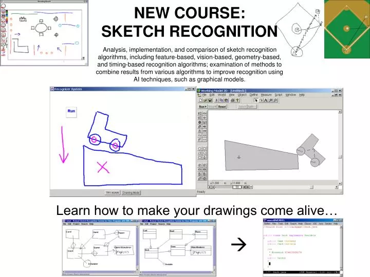
1.  NEW COURSE: SKETCH RECOGNITION Analysis, implementation, and comparison of sketch recognition algorithms, including feature-based, vision-based, geometry-based, and timing-based recognition algorithms; examination of methods to combine results from various algorithms to improve recognition using AI techniques, such as graphical models. Learn how to make your drawings come alive…

2. Sezgin • Finds corners in a polygon or in a complex shape. • First: Polygon

3. Direction Direction of each stroke segment = arctan2(dy,dx) Add check to make sure graph continuous (e.g., add 2pi)

4. Curvature Change in direction for each segment

5. Speed Speed of each segment (already computed in Rubine)

6. Threshold Curvature • Threshold = mean curvature

7. Threshold Speed • Threshold = 90% of mean

8. Select Vertices for Each • Max of all sections above threshold • Fd = curvature points

9. Select Vertices for Each • Max of all sections above threshold • Fs = speed points

10. Initial Fit • Intersection of Fd and Fs (and of course the endpoints)

11. Local neighborhood: i-k, i+k • Si is a stroke point • k is number of stroke point on either side to search • Le = Euclidian distance from Si-k to Si+k • K not defined • Lets try k = 3 … AND • Variable k where min(Le > 6 pixels)

12. Curvature Certainty Metric for Fd • di = curvature at point i • l = stroke segment curve length from Si-k to Sj+k • Lets call it CCM(vi)

13. Speed Certainty Metric for Fs • Lets call it SCM(vi)

14. Vertex Possibilities: • Fd: Possibilities based on curvature • Fs: Possibilities based on speed • CCM(Fd) : Curvature Certainty Metric • SCM(Fd) : Speed Certainty Metric • H0 = Initial Hybrid Fit = intersection of Fd and Fs (and endpoints)

15. Selecting new points to add • Hi’ = H0 + max(SCM(Fs – H0) ) • Hi’’ = H0 + max(CCM(Fd – H0)) • Pick highest scoring from each list • Try to add it to the H0

16. Make Line Segments for Hi’ and Hi’’ • For each vertex vi in Hi – create a list of line segments between vi and vi+1 • If there are n points in the vertex selection, there will be n-1 line segments

17. Calculate Errorfor Both Hi’ and Hi’’ • S = total stroke length (not Euclidean distance) • ODSQ = orthogonal distance squared • ODSQ(s,Hi) = distance of stroke point s to appropriate line segment (previous slide)

18. Distance from point to line segment • if isPointOnLine(point, line) • theDistance = 0; • else • array1 = getLineAxByC(line); • array2 = getAxByCPerpendicularLine(line, point); • A = [array1(1), array1(2); array2(1), array2(2)]; • b = [array1(3); array2(3)]; • intersectsPoint = linsolve(A, b)'; • if isPointOnLine(intersectsPoint, line) • theDistance = getLineLength([intersectsPoint; point]); • else • dist(1) = getLineLength([line(1,:); point]); • dist(2) = getLineLength([line(2,:); point]); • theDistance = min(dist); • end • end

19. Select either Hi’ or Hi’’ • Pick the one with the lower error • (in the paper this is also the one with the `higher score’ – score in this sense is just an internal ranking metric) • H1 = Hi’ or Hi’’ (the one with the lower error) • We have added one vertex point.

20. Repeat • Create new Hi’ and Hi’’ • Hi’ = H1 + max(SCM(Fs – H1) ) • Hi’’ = H1 + max(CCM(Fd – H1)) • (Note one of them will be the same as the previous time.) • Recompute error and continue

21. When to Stop • Stop when error is below the threshold. • … what is threshold? • Not in paper • Lets • Compute the error for H0 = e0 • Compute the error for Hall (all the chosen v) = eall • We want something in the middle: close to eall • .1*(e0-eall) + eall • You will try other thresholds in your implementation

22. Implications • Anything that you can describe geometrically you can build sketch system for

23. Curves • Stroke between corners can be curve or line • Is line if l2/l1 is close to 1. • Lets use .9 < l2/l1 *1.1 < 1 • Else is curve

24. Sezgin Bezier Curve Fitting • Want to replace with a Bezier curve • http://www.math.ubc.ca/people/faculty/cass/gfx/bezier.html • Bezier Demo • 2 endpoints and 2 control points

25. Bezier curve equation • http://www.cl.cam.ac.uk/Teaching/2000/AGraphHCI/SMEG/node3.html • http://www.moshplant.com/direct-or/bezier/math.html • P0 (x0,y0) = p1, P1 = c1, P2 = c2, P3 = p2 • x(t) = axt3 + bxt2 + cxt + x0 • y(t) = ayt3 + byt2 + cyt + y0 • cx = 3 (x1 - x0)bx = 3 (x2 - x1) - cxax = x3 - x0 - cx - bx • cy = 3 (y1 - y0)by = 3 (y2 - y1) - cyay = y3 - y0 - cy - by

26. Sezgin Bezier Curve Fitting • Control points • Endpoints: u = p1, v = p2 • T1= tangent vector – initial direction of stroke at point p1 • T2 = tangent vector of p2 – initial direction of stroke at point p2 • K = stroke length / 3 • 3 is common approximation • c1=k*t1 + v • c2 = k*t2 + u

27. Want to Test our Approximation • Perhaps this is really a very complex curve which can’t be fit with a simple Bezier curve • E.g., the treble clef of a musical staff • Discretize the curve. (It doesn’t say into how many parts – I leave that up to you.) • Linear approximation for each part

28. If error too high • Break our curve down the middle into two curves, and try again.

29. Matlab Curve Fitting • function [estimates, model] = fitcurvedemo(xdata, ydata) • % Call fminsearch with a random starting point. • start_point = rand(1, 2); • model = @expfun; • estimates = fminsearch(model, start_point); • % expfun accepts curve parameters as inputs, and outputs sse, • % the sum of squares error for A * exp(-lambda * xdata) - ydata, • % and the FittedCurve. FMINSEARCH only needs sse, but we want to • % plot the FittedCurve at the end. • function [sse, FittedCurve] = expfun(params) • A = params(1); • lambda = params(2); • FittedCurve = A .* exp(-lambda * xdata); • ErrorVector = FittedCurve - ydata; • sse = sum(ErrorVector .^ 2); • end • end

30. Circles and Ellipses • Least squares fit • Make a bounding box of stroke and form • Oval is formed from that bounding box. • Circle is easy: • Find out how far the circle is from the center = d, return (d-r)^2 • Ellipse more complicated

31. Project Suggestions • Build a finite state machine recognizer for the computability class to easily draw and hand in their diagrams. • Build a physics drawing program that attaches to a design simulator (we have interactive physics 2005) • Build a fashion drawing program. You draw clothes on a person, and it puts them one the person.

32. Project Ideas • Build a robot drawing and simulation program. You draw the robot and have a number of gestures to have it do different things • Gesture Tetris

33. Project Suggestions • Use both rubine and geometrical methods in recognition • Develop new ways for editing. • Build new low level recognizers

34. Projects! • Proposal due: Sept 22 • Visualization Contest • Ivc.tamu.edu/competition • Smart Boards coming • IAP (Industrial Affiliates Program) Demo

35. Projects! • 2 types: • Cool application • Sketch front end to your own research system • Fun application to go on smart board/vis contest • Gesture Tetris • TAMU gesture-based map/directory info • Computability/Physics/EE/MechEng simulator • New recognition algorithm • Significant change to old techniques to make a new application

36. Final Project Handin • Implementation… Build it… • In class Demonstration (5-10 minutes) • Previous work • Find at least 3 relevant papers (not read inc class) • Assign one for class to read, you lead short discussion • Test • Run your recognition system on data. • Find out what data you need (e.g., UML class diagrams) • Each student in class will supply others data • + Find 6 more people outside (to give 15 different people) • Paper • Introduction (why important) • Previous Work • Implementation • Results • Conclusion

37. Syllabus • http://www.cs.tamu.edu/faculty/hammond/courses/SR/2006