Download
1 / 63
630 likes | 633 Vues
This course covers advanced topics in the design of software systems and information systems, including database management systems, query optimization, distributed databases, fault tolerance techniques, and decision support systems. It also explores spatial and geographic data and introduces students to the concepts of dependability and secure computing.

E N D
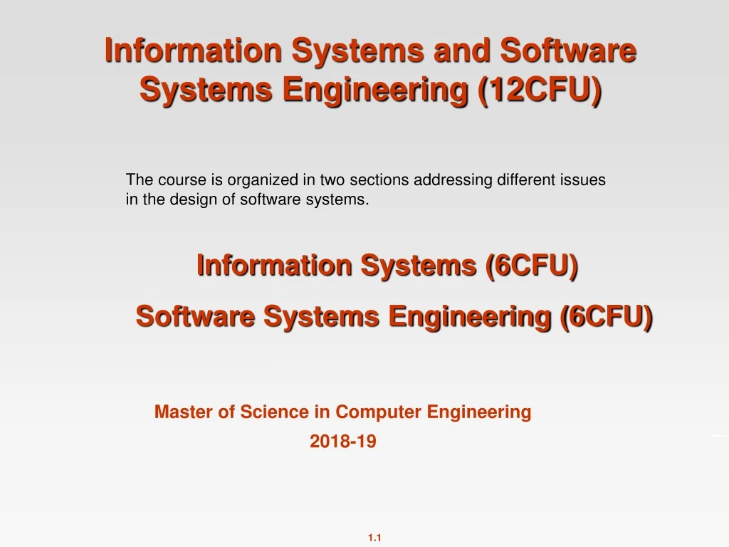
Information Systems and Software Systems Engineering (12CFU) The course is organized in two sections addressing different issues in the design of software systems. Information Systems (6CFU) Software Systems Engineering (6CFU) Master of Science in Computer Engineering 2018-19
Information Systems (6CFU) Prof. Cinzia Bernardeschi Master of Science in Computer Engineering 2018-19
The "classic" view of Information systems (IS) A computer(-based) information system is essentially an IS using computer technology to carry out some or all of its planned tasks.
Course outline Advanced database management systems topics to be used in the context of information systems • Data Storage: File Structure and Indexing • Query Optimization • Transaction management • Distributed databases • Faults, Errors, Failures: basicconcepts • Fault tolerance techniques • Stable storage implementation • Recovery System • Reliability and Availabilty measures (Mobiustool) • Spatial and Geographic data (GIS) • Decision-Support Systems: Data warehousing
Book: Silberschatz, Korth and Sudarshan Database System Concepts, McGraw-Hill Paper: AlgirdasAvizienis, Jean-Claude Laprie, et al. Basic Concepts and Taxonomy of Dependable and Secure Computing IEEE Transaction on Dependable and Secure Computing, vol. 1, n. 1, 2004 ……………………………………………………………………….. Background: Database system concepts book. Chapter 1: Introduction PART 1: Chapter 2, 3, 4 (Subs. 4.1, 4.2, 4.3, 4.4) PART 2: Chapter 6, 7 (Subs.7.1, 7.2, 7.3) Tool MySQL5.0 …………………………………………………………………………. These slides are a modified version of the slides of the book “Database System Concepts”, 5th Ed., Silberschatz, Korth and Sudarshan. Original slides are available at www.db-book.com
Database Management System (DBMS) • DBMS contains information about a particular enterprise • Collection of interrelated data (often referred to as the Data Base) • Set of programs to access the data • An environment that is both convenient and efficient to use • Database Applications: • Banking: all transactions • Airlines: reservations, schedules • Universities: registration, grades • Sales: customers, products, purchases • Online retailers: order tracking, customized recommendations • Manufacturing: production, inventory, orders, supply chain • Human resources: employee records, salaries, tax deductions
Purpose of Database Systems • In the early days, database applications were built directly on top of file systems. The system stores permanent records into files. Application programs to extract and add records to files.A file-processing-system is supported by a conventional operating system. • Drawbacks of using file systems to store data: • Data redundancy and inconsistency • Multiple file formats, duplication of information in different files(different programers created data/progr over a long period) • Difficulty in accessing data • Need to write a new program to carry out each new task • Data isolation — multiple files and formats • Integrity problems • Integrity constraints (e.g. account balance > 0) become “buried” in program code rather than being stated explicitly • Hard to add new constraints or change existing ones
Purpose of Database Systems (Cont.) • Drawbacks of using file systems (cont.) • Atomicity of updates (a computer is subject to failures) • Failures may leave database in an inconsistent state with partial updates carried out • Example: Transfer of funds from one account to another should either complete or not happen at all • Concurrent access by multiple users (for the sake of overall performance of the system) • Concurrent accessed needed for performance • Uncontrolled concurrent accesses can lead to inconsistencies • Example: Two people reading a balance and updating it at the same time • Security problems • Hard to provide user access to some, but not all, data • Database systems offer solutions to all the above problems
Levels of Abstraction A major purpose of a DBMS is to provide a user with an abstract view of data • Physical level: describes how a record (e.g., customer) is stored. • Logical level: describes data stored in database, and the relationships among the data. typecustomer = record customer_id : string; customer_name : string;customer_street : string;customer_city : integer; end; • View level: application programs hide details of data types. Views can also hide information (such as an employee’s salary) for security purposes.
View of Data An architecture for a database system
Instances and Schemas Databases change over time as information is inserted and deleted. • Similar to types and variables in programming languages • Schema – the logical structure of the database • Example: The database consists of information about a set of customers and accounts and the relationship between them) • Analogous to type information of a variable in a program • Physical schema: database design at the physical level • Logical schema: database design at the logical level • Instance – the actual content of the database at a particular point in time • Analogous to the value of a variable • Physical Data Independence – the ability to modify the physical schema without changing the logical schema • Applications depend on the logical schema • In general, the interfaces between the various levels and components should be well defined so that changes in some parts do not seriously influence others.
Data Models Underlying the structure of a data base is the data model • A collection of conceptual tools for describing • Data • Data relationships • Data semantics • Data constraints • Entity-Relationship data model (E-R is based on the perception of real world) • Relational model (uses collection of tables to represent both data and relationship among those data) • Object-based data models (Object-oriented and Object-relational) • Semistructured data model (XML- Extensible Markup Language- different data of the same type have different attributes) • Other older models: • Network model • Hierarchical model
The Entity-Relationship Model • Models an enterprise as a collection of entities and relationships • Entity: a “thing” or “object” in the enterprise that is distinguishable from other objects • Described by a set of attributes • Relationship: an association among several entities • Represented diagrammatically by an entity-relationship diagram: The key univocally identifies a record
Data Manipulation Language (DML) • Language for accessing and manipulating the data organized by the appropriate data model • DML also known as query language • Two classes of languages • Procedural – user specifies what data is required and how to get those data • Declarative (nonprocedural) – user specifies what data is required without specifying how to get those data • SQL is the most widely used query language
Data Definition Language (DDL) • Specification notation for defining the database schema Example: create tableaccount (account-numberchar(10),balanceinteger) • DDL compiler generates a set of tables stored in a data dictionary • Data dictionary contains metadata (i.e., data about data) • Database schema • Data storage and definition language • Specifies the storage structure and access methods used • Integrity constraints • Domain constraints • Referential integrity (references constraint in SQL) • Assertions • Authorization
Relational Model Attributes • Example of tabular data in the relational model Each table has multiple columns, each column has a unique name A relational database is based on the Relational model and uses a collection of tables to represent both data and relationship among those data
A Sample Relational Database which accounts belong to which customers
SQL • SQL: widely used non-procedural language • Example: Find the name of the customer with customer-id 192-83-7465select customer.customer_namefrom customerwherecustomer.customer_id = ‘192-83-7465’ • Example: Find the balances of all accounts held by the customer with customer-id 192-83-7465selectaccount.balancefromdepositor, accountwheredepositor.customer_id = ‘192-83-7465’ anddepositor.account_number = account.account_number • Application programs generally access databases through one of • Language extensions to allow embedded SQL • Application program interface (e.g., ODBC/JDBC) which allow SQL queries to be sent to a database non-procedural:“what data are needed withouth specifying how to get those data”
Database Design The process of designing the general structure of the database: • User requirements – interaction with domain experts to carry out the specification of user requirements • Conceptual design – Translate the requirements into a conceptual schemaFunctional Requirements: user defines the kinds of operations that will be performed on data. Review of the schema to meet functional requirements • Logical Design – • What attributes should we record in the database? • What relation schemas should we have and how should the attributes be distributed among the various relation schemas? • Deciding on the database schema. Database design requires that we find a “good” collection of relation schemas (no unnecessary redundancy, retrieve information easily)The most common approach is to use “functional dependencies” • Physical Design – Deciding on the physical layout of the database
Data Base Design for Banking Enterprise Major characteristics • The bank is organised into branches. Each branch is located in a particular city and is identified by a unique name. The bank monitors the assets of each branch. • Bank customers are identified by their customer_id value. The bank stores each customer’s name, and the street and the city where the customer lives. Customers may have accounts and can take out loans. A customer may be associated with a particular banker; who may act as a loan officer or personal banker for that customer. • The bank offers two types of accounts: savings and checking accounts. Accounts can be held by more than one customer, and a customer can have more than one account. Each account is assigned a unique account number. The bank mantains a record of each account’s balance and the most recent date on which the account was accessed by each customer holding the account. In addition each savings account has an interest rate, and overdrafts are recorded for each checking account.
Banking Enterprise • The bank provides its customers with loans. A loan originates at a particular branch and can be held by one or more customers. A loan is identified by unique loan number. For each loan, the bank keeps track of loan amount and the loan payments. Although a loan-payment number does not uniquely identify a particular payment among those for all the bank’s loans, a payment number does identify a particular payment for a specific loan. The date and the amount are recorded for each payment. • Bank employees are identified by their employee_id values. The bank administration stores the name and telephone number of each employee, the names of the employee’s dependents, and the employee_id number of the employee’s manager. The bank also keeps track of the employee’s start date and, thus, length of employment. To keep the example small, we do not keep track of deposits and withdrawals from savings and checking accounts, just as it keeps track of payments to loan accounts.
Entity Sets customer and loan customer_id customer_ customer_ customer_ loan_ amount name street city number
Relationship Sets (Cont.) • An attribute can also be property of a relationship set. • For instance, the depositor relationship set between entity sets customer and account may have the attribute access-date
Degree of a Relationship Set • Refers to number of entity sets that participate in a relationship set. • Relationship sets that involve two entity sets are binary (or degree two). Generally, most relationship sets in a database system are binary. • Relationship sets may involve more than two entity sets. • Relationships between more than two entity sets are rare. Most relationships are binary. (More on this later.) • Example: Suppose employees of a bank may have jobs (responsibilities) at multiple branches, with different jobs at different branches. Then there is a ternary relationship set between entity sets employee, job, and branch
Attributes • An entity is represented by a set of attributes, that is descriptive properties possessed by all members of an entity set. • Domain – the set of permitted values for each attribute • Attribute types: • Simple and composite attributes. • Single-valued and multi-valued attributes • Example: multivalued attribute: phone_numbers • Derived attributes • Can be computed from other attributes • Example: age, given date_of_birth Example: customer = (customer_id, customer_name, customer_street, customer_city ) loan = (loan_number, amount )
E-R Design Decisions • The use of an attribute or entity set to represent an object. • Whether a real-world concept is best expressed by an entity set or a relationship set. • The use of a ternary relationship versus a pair of binary relationships. • The use of a strong or weak entity set. • The use of specialization/generalization – contributes to modularity in the design. • The use of aggregation – can treat the aggregate entity set as a single unit without concern for the details of its internal structure.
Reduction to Relation Schemas • Primary keys allow entity sets and relationship sets to be expressed uniformly as relation schemas that represent the contents of the database. • A database which conforms to an E-R diagram can be represented by a collection of schemas. • For each entity set and relationship set there is a unique schema that is assigned the name of the corresponding entity set or relationship set. • Each schema has a number of columns (generally corresponding to attributes), which have unique names.
The Banking Schema • branch = (branch_name, branch_city, assets) • customer = (customer_id, customer_name, customer_street, customer_city) • loan = (loan_number, amount) • account = (account_number, balance) • employee = (employee_id. employee_name, telephone_number, start_date) • dependent_name = (employee_id, dname) • account_branch = (account_number, branch_name) • loan_branch = (loan_number, branch_name) • borrower = (customer_id, loan_number) • depositor = (customer_id, account_number) • cust_banker = (customer_id, employee_id, type) • works_for = (worker_employee_id, manager_employee_id) • payment = (loan_number, payment_number, payment_date, payment_amount) • savings_account = (account_number, interest_rate) • checking_account = (account_number, overdraft_amount)
Representing Entity Sets as Schemas • A strong entity set reduces to a schema with the same attributes. • A weak entity set becomes a table that includes a column for the primary key of the identifying strong entity set payment = ( loan_number, payment_number, payment_date, payment_amount )
Representing Relationship Sets as Schemas • A many-to-many relationship set is represented as a schema with attributes for the primary keys of the two participating entity sets, and any descriptive attributes of the relationship set. • Example: schema for relationship set borrower borrower = (customer_id, loan_number )
Storage Access • A database file is partitioned into fixed-length storage units called blocks. Blocks are units of both storage allocation and data transfer. • Database system seeks to minimize the number of block transfers between the disk and memory. We can reduce the number of disk accesses by keeping as many blocks as possible in main memory. • Buffer– portion of main memory available to store copies of disk blocks. • Buffer manager – subsystem responsible for allocating buffer space in main memory.
Buffer Manager • Programs call on the buffer manager when they need a block from disk. • If the block is already in the buffer, buffer manager returns the address of the block in main memory • If the block is not in the buffer, the buffer manager • Allocates space in the buffer for the block • Replacing (throwing out) some other block, if required, to make space for the new block. • Replaced block written back to disk only if it was modified since the most recent time that it was written to/fetched from the disk. • Reads the block from the disk to the buffer, and returns the address of the block in main memory to requester.
Buffer-Replacement Policies • Most operating systems replace the block least recently used (LRU strategy) • Idea behind LRU – use past pattern of block references as a predictor of future references • Queries have well-defined access patterns (such as sequential scans), and a database system can use the information in a user’s query to predict future references • LRU can be a bad strategy for certain access patterns involving repeated scans of data • For example: when computing the join of 2 relations r and s by a nested loops for each tuple tr of r do for each tuple ts of s do if the tuples tr and ts match … • Mixed strategy with hints on replacement strategy providedby the query optimizer is preferable
Buffer-Replacement Policies (Cont.) • Pinned block – memory block that is not allowed to be written back to disk. • Toss-immediate strategy – frees the space occupied by a block as soon as the final tuple of that block has been processed • Most recently used (MRU) strategy – system must pin the block currently being processed. After the final tuple of that block has been processed, the block is unpinned, and it becomes the most recently used block. • Buffer manager can use statistical information regarding the probability that a request will reference a particular relation • E.g., the data dictionary is frequently accessed. Heuristic: keep data-dictionary blocks in main memory buffer • Buffer managers also support forced output of blocks for the purpose of recovery (more in Chapter 17)
File Organization • The database is stored as a collection of files. Each file is a sequence of records. A record is a sequence of fields. • One approach: • assume record size is fixed • each file has records of one particular type only • different files are used for different relations This case is easiest to implement; will consider variable length records later.
Fixed-Length Records • Simple approach: • Store record i starting from byte n (i – 1), where n is the size of each record. • Record access is simple but records may cross blocks • Modification: do not allow records to cross block boundaries • Deletion of record i: alternatives: • move records i + 1, . . ., nto i, . . . , n – 1 • move record n to i • do not move records, but link all free records on afree list
Free Lists • Store the address of the first deleted record in the file header. • Use this first record to store the address of the second deleted record, and so on • Can think of these stored addresses as pointerssince they “point” to the location of a record. • More space efficient representation: reuse space for normal attributes of free records to store pointers. (No pointers stored in in-use records.)
Variable-Length Records • Variable-length records arise in database systems in several ways: • Storage of multiple record types in a file. • Record types that allow variable lengths for one or more fields. • Record types that allow repeating fields (used in some older data models).
Variable-Length Records: Slotted Page Structure • Slotted page header contains: • number of record entries • end of free space in the block • location and size of each record • Records can be moved around within a page to keep them contiguous with no empty space between them; entry in the header must be updated. • Pointers should not point directly to record — instead they should point to the entry for the record in header.