Download
1 / 30
300 likes | 446 Vues
Modelling multiple sample selection in intergenerational occupational mobility. Cheti Nicoletti ISER, University of Essex Marco Francesconi Department of Economics, University of Essex. Main aim s of the paper. Estimation of intergenerational occupational mobility in Britain.

E N D
Modelling multiple sample selection in intergenerational occupational mobility Cheti Nicoletti ISER, University of Essex Marco Francesconi Department of Economics, University of Essex
Main aims of the paper • Estimation of intergenerational occupational mobility in Britain. 2. Correcting for potential sample selection problems in short panels using different estimation methods.
Sample selection problems • Labour market selection: Intergenerational occupational mobility can be estimated only for people who are employed. • Coresidence selection: Children must be living together with their parents in at least one wave of the panel.
BHPS 1991-1993 1991 1997 2003 Cohort 1988 1983 1978 1973 1968 1963 1958 Child age 3 8 13 18 23 28 33 Child age 9 14 19 24 29 34 39 Child age 15 20 25 30 35 44 45
Taking account of coresidence selection Francesconi and Nicoletti (2006) find that the intergenerational mobility in occupational prestige is underestimated when using the subsample of sons born between 1966 and 1985. They try different estimation methods to correct for sample selection and find that only the inverse propensity score is able to attenuate the selection problem This sample selection evaluation is possible because all BHPS respondents are asked to report occupational characteristics of their parents when they were 14
Taking account of selection into employment for children • Blanden (2005) and Ermisch et al (2005) consider two-step estimation procedures and find lower and unchangedβs • Couch and Lillard (1998) and Nicoletti and Francesconi (2006) consider imputation methods and find lowerβs • Minicozzi (2003) use partial identification approach to produce bound estimates instead than point estimates for the intergenerational mobility and find higherβs when including unemployed and part-time workers.
Contributions of the paper • Propose new estimation methods to take account of sample selection problem in the intergenerational mobility models which are very parsimonious • Taking account of both coresidence and employment selection bias
Selection models • If εi and ui are not independent then we have selection due to unobservables • If εi depends on Zi then we have selection due to observables • If εi depends on Zi and ui then we have selection due to both observables and unobservables
Selection due to unobservables y=α+xβ+εd*=Z γ+ud=l(d*>0) • Let E(ε|x)=0, ε ind Z, (ε,u) be N with means zeros, variances σ2 and 1 and covariance ρ • Then E((y-α-xβ) |x,d=1) ≠ 0 and OLSE is biased • E(y|x,d=1)=α+xβ+E(ε|x,d=1)=α+xβ+ ρλ • v=ε- ρλis such that E(v|d=1,X)=0 • We can consider an additional correction term (Heckman 1979, Vella 1998)
Selection due to observables y=α+xβ+εd*=Z γ+ud=l(d*>0) • Let E(ε|x)=0, ε ╨ u but ε not ind Z • Then E(ε|x,d=1)≠0 and OLSE is biased because of selection on observables • Since ε ╨ d|x,Z we can adopt (1) propensity score methods, (2) regression adjustment methods or (3) combining methods. (seeRosembaum and Rubin, 1983; Robins and Rotnitzky, 1995; Hirano et al., 2003)
Propensity score weighting method Let Pr(d=1|x,Z)=Pr(d=1|Z)=p(Z) Then E(ε d|x) ≠ 0 butE(ε d p(Z)-1|x)=0 E(ε d p(Z)-1|x)= EZE(ε d p(Z)-1|x,Z) = EZ[E(ε |x,Z,d=1) Pr(d=1|x,Z)p(Z)-1] Since ε ╨ d|x,Z =EZ[E(ε |x,Z) Pr(d=1|x,Z)p(Z)-1] =EZ[E(ε |x,Z)]=E(ε |x)=0 This holds even if some of the variables in Z are erroneously omitted from the main equation.
Regression adjustment y=α+xβ+εd*=Z γ+ud=l(d*>0) • To take account that ε is not ind of Z y=αN+xβN+Zδ+ω • Ifthe linearity assumption is satisfied then E(ω|X,Z,d=1)=E(ω|X,Z)=E(ω|X)=0 and • βN is consistently estimated • β=Cov(x,y)/Var(x)=βN+Cov(x,Z)Var(Z)-1δ
Combining regression adjustment and propensity score method Estimation of the extended model y=α+xβ+Zδ+ω by using inverse propensity score weighting E[(y-α-xβ-Zδ) d p(Z)-1|x] = EZE[(y-α-xβ- Zδ) d p(Z)-1|x,Z] = EZ[E(y-α-xβ- Zδ |x,Z,d=1) Pr(d=1|x,Z)p(Z)-1] Notice that this expression is 0 if either E(y-α-xβ- Zδ |x,Z,d=1)=E(ω|X,Z,d=1)=0 or Pr(d=1|x,Z)=p(Z) holds and not necessarily both.
Selection due to both observables and unobservables y=α+xβ+εd*=Z γ+ud=l(d*>0) where εdepends on both Z and u (ε,u) is N with means zeros, variances σ2 and 1 and covariance ρ v=(ε- ρλ) ind d |x,Z We can use: (1) Heckman correction and propensity score weighting or (2) Heckman correction and regression adjustment.
Heckman correction & propensity score weighting E[(y-α-xβ- ρλ) d p(Z)-1|x] = EZE[(y-α-xβ- ρλ) d p(Z)-1|x,Z] = EZ[E(y-α-xβ- ρλ|x,Z,d=1) Pr(d=1|x,Z)p(Z)-1] Since (y-α-xβ- ρλ)╨ d|x,Z =EZ[E(y-α-xβ- ρλ |x,Z) Pr(d=1|x,Z)p(Z)-1] =EZ[E(y-α-xβ- ρλ |x,Z)]= E(y-α-xβ- ρλ |x)= 0
Heckman correction & regression adjustment Estimation of the extended model with additional variables Z and correction termλ y=α+xβ+Zδ+ ρλ +ω d*=Z γ+u • ρλcontrols for the dependence ofε1on u • Zδcontrols for the dependence ofε2on Z
All BHPS respondents are asked to report occupational characteristics of their parents when they were 14 THEREFORE We know the occupational prestige even for daughters and fathers living apart during the panel. We can estimate the intergenerational mobility without any coresidence selection. We can consider the subsample of daughters coresident with the fathers at least once during the panel and assess the relevance of the coresidence selection. We can then compare different methods to correct for the coresidence selection. How can the BHPS help us?
BHPS Samples • FULL SAMPLE: 2691 women (daughters) born between 1966 and 1985 with at least one valid interview over the first 13 waves of the BHPS (aged between 16-37, average 24) • RESTRICTED SAMPLE: 745 individuals from the full sample who can be matched with their father (aged between 16-37, average age 21). • We consider an average occupational prestige over all waves available for daughters. We consider instead the occupation prestige reported retrospectively by daughters for fathers (average age 46).
Estimation Methods Used • Inverse propensity score weighting (Weights) • Regression adjustment • Regression adjustment & weights • Heckman correction method (Heckman) • Heckman & weights • Regression adjustment & Heckman
Coresidence selection model y=α+xβ+Aμ+εd*=Z γ+ud=l(d*>0) where y is the daughter’s occupational prestige (log Hope-Goldthorpe score) x is her father’s occupational prestige A age and age2 d=1 for daughters living together with their father in at least one wave and 0 otherwise Z=dummies for education, age, regions, ethnicity, religiosity and two house price indexes
The intergenerational equation is too parsimonious y=α+xβ+Aμ+εd*=Z γ+ud=l(d*>0) Education dummies are important to explaining both the daughters occupational prestige and their probability to be coresident The assumption that ε ╨ d is not acceptable.
Regression adjustment when x is missing y=αN+xβN+Zδ+ω • Ifthe linearity assumption is satisfied • βN is consistently estimated • β=Cov(x,y)/Var(x)=βN+Cov(x,Z)Var(Z)-1δ • If x is missing it is not possible to estimate Cov(x,Z) consistently
Employment selection model y=α+xβ+Aμ+εd*=Z γ+ud=l(d*>0) where y is the daughter’s occupational prestige (log Hope-Goldthorpe score) x is her father’s occupational prestige A age and age2 d=1 for daughters are employed at least in at least one wave and 0 otherwise Z=occupation prestige father, dummies for education, age, regions, ethnicity, religiosity, a house price index, marital status and number of children aged between 0-2, 3-4, 5-11, 12-15, 16-18.
Correcting for employment and sample selection simultaneously
Conclusions • The intergenerational equation is too parsimonious and there are probably omitted variables such as education dummies. • In this situation correcting for selection on observables is much more important than correcting for selection on unobservables. • The coresidence selection seems to cause an underestimation of β. • The selection into employment does not seem to cause a large bias in β.