Download

1 / 70
710 likes | 1.19k Vues
Chapter 16. LABOR MARKETS. CONTENTS. Allocation of Time A Mathematical Analysis of Labor Supply Market Supply Curve for Labor Labor Market Equilibrium Labor Unions. Profit Maximization and Input Demand. A firm’s output is determined by the amount of inputs it chooses to employ

E N D
Chapter 16 LABOR MARKETS
CONTENTS • Allocation of Time • A Mathematical Analysis of Labor Supply • Market Supply Curve for Labor • Labor Market Equilibrium • Labor Unions
Profit Maximization and Input Demand • A firm’s output is determined by the amount of inputs it chooses to employ • the relationship between inputs and outputs is summarized by the production function • A firm’s economic profit can also be expressed as a function of inputs (k,l) = pq –C(q) = pf(k,l) – (vk + wl)
Profit Maximization and Input Demand • The first-order conditions for a maximum are /k = p[f/k] – v = MPRK-v=0 /l = p[f/l] – w = MPRl-w= 0 • A profit-maximizing firm should hire any input up to the point at which its marginal contribution to revenues is equal to the marginal cost of hiring the input
Allocation of Time • Individuals must decide how to allocate the fixed amount of time they have • We will initially assume that there are only two uses of an individual’s time • engaging in market work at a real wage rate of w • leisure (nonwork)
Allocation of Time • Assume that an individual’s utility depends on consumption (c) and hours of leisure (h) utility = U(c,h) • In seeking to maximize utility, the individual is bound by two constraints l + h = 24 c = wl
Allocation of Time • Combining the two constraints, we get c = w(24 – h) c + wh = 24w • An individual has a “full income” of 24w • may spend the full income either by working (for real income and consumption) or by not working (enjoying leisure) • The opportunity cost of leisure is w
Utility Maximization • The individual’s problem is to maximize utility subject to the full income constraint • Setting up the Lagrangian L = U(c,h) + (24w – c – wh) • The first-order conditions are L/c = U/c - = 0 L/h = U/h - = 0
Utility Maximization • Dividing the two, we get • To maximize utility, the individual should choose to work that number of hours for which the MRS (of h for c) is equal to w • to be a true maximum, the MRS (of h for c) must be diminishing
Income andSubstitution Effects • Both a substitution effect and an income effect occur when w changes • when w rises, the price of leisure becomes higher and the individual will choose less leisure • because leisure is a normal good, an increase in w leads to an increase in leisure • The income and substitution effects move in opposite directions (now, an individuals are supplier of labor)
Income andSubstitution Effects Consumption The substitution effect is the movement from point A to point C The income effect is the movement from point C to point B B C The individual chooses less leisure as a result of the increase in w A U2 U1 Leisure substitution effect > income effect
Income andSubstitution Effects Consumption The substitution effect is the movement from point A to point C The income effect is the movement from point C to point B The individual chooses more leisure as a result of the increase in w B C A U2 U1 Leisure substitution effect < income effect
A Mathematical Analysisof Labor Supply (omitted)
A Mathematical Analysisof Labor Supply • We will start by amending the budget constraint to allow for the possibility of nonlabor income c = wl + n • Maximization of utility subject to this constraint yields identical results • as long as n is unaffected by the labor-leisure choice
A Mathematical Analysisof Labor Supply • The only effect of introducing nonlabor income is that the budget constraint shifts out (or in) in a parallel fashion • We can now write the individual’s labor supply function as l(w,n) • hours worked will depend on both the wage and the amount of nonlabor income • since leisure is a normal good, l/n < 0
Dual Statement of the Problem • The dual problem can be phrased as choosing levels of c and h so that the amount of expenditure (E = c – wl) required to obtain a given utility level (U0) is as small as possible • solving this minimization problem will yield exactly the same solution as the utility maximization problem
Dual Statement of the Problem • A small change in w will change the minimum expenditures required by E/w = -l • this is the extent to which labor earnings are increased by the wage change
Dual Statement of the Problem • This means that a labor supply function can be calculated by partially differentiating the expenditure function • because utility is held constant, this function should be interpreted as a “compensated” (constant utility) labor supply function lc(w,U)
Slutsky Equation ofLabor Supply • The expenditures being minimized in the dual expenditure-minimization problem play the role of nonlabor income in the primary utility-maximization problem lc(w,U) = l[w,E(w,U)] = l(w,N) • Partial differentiation of both sides with respect to w gives us
Slutsky Equation ofLabor Supply • Substituting for E/w, we get • Introducing a different notation for lc , and rearranging terms gives us the Slutsky equation for labor supply:
Cobb-Douglas Labor Supply • Suppose that utility is of the form • The budget constraint is c = wl + n and the time constraint is l + h = 1 • note that we have set maximum work time to 1 hour for convenience
Cobb-Douglas Labor Supply • The Lagrangian expression for utility maximization is L = ch + (w + n - wh - c) • First-order conditions are L/c = c-h - = 0 L/h = ch- - w = 0 L/ = w + n - wh - c = 0
Cobb-Douglas Labor Supply • Dividing the first by the second yields
Cobb-Douglas Labor Supply • Substitution into the full income constraint yields c = (w + n) h = (w + n)/w • the person spends of his income on consumption and = 1- on leisure • the labor supply function is
Cobb-Douglas Labor Supply • Note that if n = 0, the person will work (1-) of each hour no matter what the wage is • the substitution and income effects of a change in w offset each other and leave l unaffected
Cobb-Douglas Labor Supply • If n> 0, l/w > 0 • the individual will always choose to spend n on leisure • Since leisure costs w per hour, an increase in w means that less leisure can be bought with n
Cobb-Douglas Labor Supply • Note that l/n < 0 • an increase in nonlabor income allows this person to buy more leisure • income transfer programs are likely to reduce labor supply • lump-sum taxes will increase labor supply
CES Labor Supply • Suppose that the utility function is • Budget share equations are given by • where = /(-1)
CES Labor Supply • Solving for leisure gives and
w* lB* l* lA* lA* + lB* = l* Market Supply Curve for Labor To derive the market supply curve for labor, we sum the quantities of labor offered at every wage Individual A’s supply curve w w Individual B’s supply curve w sA Total labor supply curve S sB l l l
Market Supply Curve for Labor Note that at w0, individual B would choose to remain out of the labor force Individual A’s supply curve w w Individual B’s supply curve w sA Total labor supply curve S sB w0 l l l As w rises, l rises for two reasons: increased hours of work and increased labor force participation
Labor Market Equilibrium • Equilibrium in the labor market is established through the interactions of individuals’ labor supply decisions with firms’ decisions about how much labor to hire
At w*, the quantity of labor demanded is equal to the quantity of labor supplied w* l* Labor Market Equilibrium “sticky” real wages-Macoeconomics real wage At any wage above w*, the quantity of labor demanded will be less than the quantity of labor supplied S=AE At any wage below w*, the quantity of labor demanded will be greater than the quantity of labor supplied D=MRP quantity of labor
Mandated Benefits • A number of new laws have mandated that employers provide special benefits to their workers • health insurance • paid time off • minimum severance packages • The effects of these mandates depend on how much the employee values the benefit
Mandated Benefits • Suppose that, prior to the mandate, the supply and demand for labor are lS = a + bw lD = c – dw • Setting lS = lD yields an equilibrium wage of w* = (c – a)/(b + d)
Mandated Benefits • Suppose that the government mandates that all firms provide a benefit to their workers that costs t per unit of labor hired • unit labor costs become w + t • Suppose also that the benefit has a value of kper unit supplied • the net return from employment rises to w + k
Mandated Benefits • Equilibrium in the labor market then requires that a + b(w + k) = c – d(w + t) • This means that the net wage is
Mandated Benefits • If workers derive no value from the mandated benefits (k = 0), the mandate is just like a tax on employmentw and l all decrease • similar results will occur as long as k < t • If k = t, the new wage falls precisely by the amount of the cost and the equilibrium level of employment does not change
Mandated Benefits • If k > t, the new wage falls by more than the cost of the benefit and the equilibrium level of employment risesw decrease and L increase
Wage Variation • It is impossible to explain the variation in wages across workers with the tools developed so far • we must consider the heterogeneity that exists across workers and the types of jobs they take
Wage Variation • Human Capital • differences in human capital translate into differences in worker productivities • workers with greater productivities would be expected to earn higher wages • while the investment in human capital is similar to that in physical capital, there are two differences • investments are sunk costs • opportunity costs are related to past investments
Wage Variation • Compensating Differentials • individuals prefer some jobs to others • desirable job characteristics may make a person willing to take a job that pays less than others • jobs that are unpleasant or dangerous will require higher wages to attract workers • these differences in wages are termed compensating differentials
Monopsony in theLabor Market • In many situations, the supply curve for an input (l) is not perfectly elastic • We will examine the polar case of monopsony, where the firm is the single buyer of the input in question • the firm faces the entire market supply curve • to increase its hiring of labor, the firm must pay a higher wage
Monopsony in theLabor Market&&& • The marginal expense (ME) associated with any input is the increase in total costs of that input that results from hiring one more unit • if the firm faces an upward-sloping supply curve for that input, the marginal expense will exceed the market price of the input
Monopsony in theLabor Market • If the total cost of labor is wl, then • In the competitive case, w/l = 0 and MEl = w • If w/l > 0, MEl > w
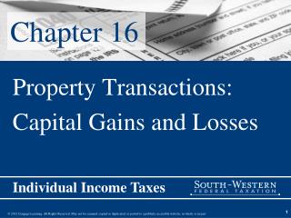
Note that the quantity of labor demanded by this firm falls short of the level that would be hired in a competitive labor market (l*) The wage paid by the firm will also be lower than the competitive level (w*) w* w1 l1 l* Monopsony in theLabor Market Wage MEl S D Labor
Monopsonistic Hiring • Suppose that a coal mine’s workers can dig 2 tons per hour and coal sells for $10 per ton • this implies that MRPl = $20 per hour • If the coal mine is the only hirer of miners in the local area, it faces a labor supply curve of the form l = 50w