Download
1 / 80
820 likes | 1.17k Vues
Chapter 8: Aggregate Demand and Aggregate Supply. The aggregate demand schedule The aggregate supply schedule Long run aggregate supply Short run aggregate supply Equilibrium in the AD-AS Model Comparative statics in the AD-AS model Aggregate demand shocks Aggregate supply shocks

E N D
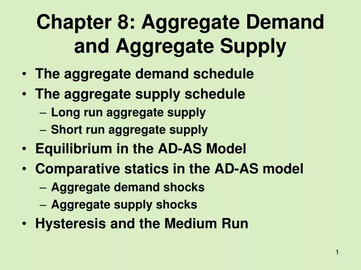
Chapter 8: Aggregate Demand and Aggregate Supply • The aggregate demand schedule • The aggregate supply schedule • Long run aggregate supply • Short run aggregate supply • Equilibrium in the AD-AS Model • Comparative statics in the AD-AS model • Aggregate demand shocks • Aggregate supply shocks • Hysteresis and the Medium Run
Learning Objectives • Understand the relation between prices and aggregate demand • To determine the non-accelerating inflation rate of unemployment (NAIRU) and the long run aggregate supply for an economy • To identify the factors that lead to shifts in the long run aggregate supply curve • To acknowledge that in the short run output can deviate from its long run equilibrium level by moving along a short run aggregate supply curve. • Understanding the difference between adaptive and rational expectations formation. • Construct the AD-AS model and use it in comparative statics exercises.
AD-AS Model • The Aggregate Demand and Aggregate Supply(AD-AS) model simultaneously determines output and prices. • This model simply aggregates across all goods and services, in which case, we are determining the average price level and the total level of output in the economy. The model is useful to policy makers who have in recent decades become increasingly concerned with how prices are determined, as well as output. • The AD-AS model shares many common features with the IS-LM model, particularly the Neoclassical version, but is more rigorous.
The aggregate demand schedule • The AD schedule plots the relationship between the price level and aggregate demand. Its construction comes directly from the IS-LM model – all we have to do is think about what happens to planned expenditures when prices fall. • When the IS-LM model is in equilibrium, planned expenditures are equal to actual output, so all we need to do is identify the effect of falling prices on the equilibrium level of output. • The combinations of prices and output can be plotted to form the downward sloping Aggregate Demand (AD) schedule.
The AD curve • The AD curve just tells us what the level of aggregate demand or planned expenditures is at each price level. • Changes in the price level will relate to movements along the curve. • However, if aggregate demand were to change due to a factor other than prices, the AD curve would shift. Shifts in the AD curve result from anything that shifts the IS or LM curve, other than a change in the price level.
The aggregate supply schedule • The Aggregate Supply (AS) schedule plots the relationship between the output of an economy and the price level. In essence, it sums all the output decisions by productive agents in the domestic economy. • An important distinction, though, exists between aggregate supply in the short and the long run. Output in the short run can deviate from its long run level if markets are in disequilibrium for a period of time because wages and prices adjust slowly towards equilibrium values.
Long run aggregate supply • In the long run, the supply decisions of firms are independent of prices. Prices are considered to be a nominal factor, whereas production decisions will be based on real concerns. We will see that these might include productivity, labour force participation, product market conditions, or factors determining the bargaining power of labour. • Long run aggregate supply is fixed at the long run equilibrium level of output, which in turn corresponds to the level of output consistent with equilibrium in the labour market. This level of output is often referred to as the natural level of output.
Long run aggregate supply • Establishing the equilibrium level of output therefore requires us to investigate the equilibrium in the labour market. • More specifically, we will be concerned with the equilibrium rate of unemployment, which is often referred to as the non-accelerating inflation rate of unemployment or the NAIRU. At this rate, there is no pressure on wages to change. And, as prices are simply a mark up on wage costs, it must also be the case that there is no pressure on prices to change either.
The equilibrium rate of unemployment or NAIRU • This refers to the rate of unemployment where the labour market is in equilibrium. • This equilibrium is considered to be the outcome of bargaining between labour (sometimes organised bodies, such as trade unions) and firms. • Bargaining works by assuming that workers are concerned with setting wages and firms with setting prices.
The wage setting curve • This schedule determines the nominal wage (W) desired by labour, and can be written as: • There are three factors which determine the wage (W) that workers will push for: • Pe are expectations of the price level. If workers anticipate higher prices, then the purchasing power of their wages will be reduced. Therefore, they would push for higher nominal wages so as to maintain the value of their real wages (purchasing power of wages).
The wage setting curve • u is the unemployment rate and exerts a negative force on wage demands. The reserve army of the unemployed are taken to be the surplus labour that is available to employers. The larger this pool becomes, the more moderate wage demands will be. Workers know that if they push for too higher wages they may be substituted for cheaper unemployed labour. Also, when unemployment is high, workers anticipate that finding new employment when unemployed will be much trickier. This forms a powerful incentive to avoid becoming unemployed in the first place by moderating wage demands. The converse is also true. At low levels of unemployment, workers would be more confident in pushing for higher wages.
The wage setting curve • Z is really a catch all variable which consists of a number of items that may influence wage demands. • The first are those factors which influence the bargaining power of workers. Trade unions bargaining collectively or employment laws giving rights to workers would be examples. • The second consists of items which raise the opportunity cost of working. For example, if unemployment benefits were relatively generous, then the costs of unemployment would be correspondingly lower which would lead to more ambitious wage demands.
The wage setting curve • For simplicity, it is assumed that workers form correct expectations concerning the price level, then Pe=P. The wage setting relationship can be expressed in terms of the real wage: • The bargained real wage falls as unemployment rises. Changes in Z would lead to shifts in the entire function, meaning that at each level of unemployment workers would target a different real wage. • The wage setting relationship is also known as the bargained real wage (BRW), as it is the real wage that unions demand in their bargaining with employers (firms).
Price-setting relationship • Firms are simply assumed to set prices as a mark up on wage costs. Although in the real world, firms will face other costs such as rents and interest payments on capital, these can be ignored in this simple model: • where μ is the mark up and LP is labour productivity. • Costs are given by the ratio of wages (W) to labour productivity (LP). Firm costs will rise if either wages rise, or labour productivity falls. If both move in the same proportion, then costs will remain unchanged.
Price-setting relationship • The mark up μ is largely determined by product market conditions, which primarily refer to the degree of competition in the market. • Where markets are relatively competitive, the mark up would be expected to be low, and under perfectly competitive conditions it would be expected to be zero (which means that firms set prices equal to marginal costs and only make normal profits). When firms can exert significant market power, the mark up would of course rise and firms would take more of a profit margin on their sales. One factor which might be crucial in determining the size of the mark up could be the level of competition policy in existence and how strongly it is enforced.
Price-setting relationship • The price-setting relationship above can be rearranged so it is also expressed in terms of the real wage: • The price setting function has been drawn as a horizontal line indicating that price-setting is independent of the level of unemployment. This makes the model easier to use, but is in itself is a debatable proposition. Some discussion justifying this assumption is presented in Global Applications 8.1.
Price-setting relationship • The price setting relationship is also known as the feasible real wage (FRW), as it states the real wage that firms can afford to pay workers given the productivity of labour and product market conditions. If there is movement in either of these two fields, then the feasible real wage will change and the price-setting schedule will shift. • An increase in labour productivity would increase the feasible real wage and hence the price-setting schedule will shift upwards. • An increase in the mark up would lower the price-setting schedule.
Equilibrium • The equilibrium rate of unemployment or the NAIRU is where the price-setting and wage-setting curves intersect. This is simply where the bargained and feasible real wages are consistent with one another. • The dynamics of this model will always move toward the equilibrium level of unemployment. Any level of unemployment away from this would induce changes in either or both wages and prices, so that the real wage and unemployment are restored to their equilibrium values.
From the equilibrium rate of unemployment to equilibrium level of output: Deriving the long run aggregate supply curve (LRAS) • The relationship between output and employment (N) is given by a production function: Y=F(N). • This simply defines the aggregate level of output for each level of employment, but can also be written in terms of the unemployment rate. The total labour force (L) consists of employed (N) and unemployed workers (U): L=N+U. • The unemployment rate is the proportion of the labour force that is unemployed: u=U/L.
Deriving the LRAS • Therefore, the proportion of the labour force that is employed and unemployed should just add up to one: 1=N/L+U/L, 1=N/L+u. • This can be rearranged to give employment as a function of the unemployment rate: N/L=1-u, N=L(1-u). • The level of employment is equal to the proportion of the labour force (L) that is not unemployed. If the unemployment rate is u, then this proportion will be equal to 1-u.
Deriving the LRAS • Finally, to find the equilibrium level of output, all we need to do is substitute this relationship between employment and unemployment back into the production function: • Shifts in the long run aggregate supply schedule will result from anything that acts to alter the equilibrium level of output.
LRAS and NAIRU • This should make it clear why the equilibrium level of unemployment is referred to as the NAIRU. • It is the rate of unemployment where there is no pressure on prices to change. • The equilibrium level of output, which then defines the position of the long run aggregate supply curve, is just the level of output at the NAIRU.
Shifts in LRAS • These shifts in long run AS can come from four sources: • Labour productivity, LP: As labour productivity improves, the equilibrium rate of unemployment falls and equilibrium employment and output both rise. As a result, the long run AS schedule will shift to the right. As a consequence of higher productivity, the price setting schedule shifts upwards. The equilibrium rate of unemployment falls, the equilibrium level of output rises, and the long run aggregate supply curve shifts to the right.
Shifts in LRAS • μ: An increase in the mark up increases the natural rate of unemployment and leads to a leftward shift in the aggregate supply schedule. An increase in the mark up would produce a downward shift in the price-setting curve and ultimately a shift in the long run aggregate supply curve. When firms increase their margins, they are increasing the average price level in the economy. At higher prices, aggregate demand will be lower, and therefore lower output and employment is sustainable. (See above figure). • Z: If the wage setting schedule shifts upwards because unemployment benefits have risen, trade unions have greater power, etc., the natural rate of unemployment rises and the long run AS schedule will shift to the left.
Shifts in LRAS • L: As the labour force increases, there are more available labour resources with which to produce output so the long run AS schedule shifts to the right. When the labour force increases, it implies that at every rate of unemployment below 100%, the level of employment will be higher. This is why the function which relates the level of employment to the rate of unemployment will shift upwards with an increase in the labour supply.
Supply side policies • Shifting the long run aggregate supply function to the right is an important goal in policy making, as the equilibrium level of output increases. From this analysis, it is clear that there are a range of policies that the government may undertake to achieve this. • Policies to improve productivity (higher LP). • Policies to improve labour market flexibility/competition (lower Z). • Policies to induce higher labour market participation (higher L). • Policies to improve product market competition (lower mark up). • Taken collectively, attempts to shift the long run aggregate supply curve are known as supply side policies. • Global Applications 2.2 Mrs. Thatcher’s supply side revolution
Short run aggregate supply • In the long run, the willingness of firms to produce does not depend on the price level, and therefore the aggregate supply function is vertical. • Aggregate supply in the short run, though, is different. In this case, it is argued that the schedule is upward-sloping, so supply rises with prices. This is how we would expect a conventional supply curve to look. • To accept an aggregate supply function which slopes upwards with prices means that we must justify why output can or might deviate from its equilibrium level. Also, as output is always expected to eventually return to its equilibrium level, we have to reason why these deviations are only temporary.
Short run aggregate supply • There are two reasons for the slope of the SRAS: • If wages and prices move slowly, then output will be away from the equilibrium level for some time. Accounting for wage and price rigidities is important. • Also important is the role that is played by expectations. When deriving the long run equilibrium level of output, we assumed that price expectations were made correctly. In the short run, though, actual prices can deviate from expected prices. This too accounts for why aggregate supply may differ in the short and long run. We will also observe that the way expectations are formed will play a critical role in the dynamics that link the short and long run.
Short run aggregate supply • One of the key features of the short run aggregate supply function is that output and prices are positively related. As output increases, then prices will also rise. • To understand what factors might be responsible for this relationship, we need to consider how prices are actually determined – a process which we have already argued is summarised by the price-setting behaviour of firms.
Short run aggregate supply • From the price-setting relationship, prices are a mark up on wage costs: • The level of wages is derived from the wage setting relationship: • If we substitute the wage setting equation into the price setting equation, we have an equation of prices determination in the economy:
Short run aggregate supply • The price-setting equation consists of a number of variables. These factors can in turn be split into long run and short run determinants of the price level. • We have already seen that changes in labour productivity, labour supply factors, and the mark up will lead to shifts in the long run aggregate supply curve. For this reason, we can ignore these as determining prices in the short run because any change in these variables will lead to a change in the equilibrium level of output. • The two remaining variables are the level of unemployment (which is strongly linked to output) and the level of price expectations.
Unemployment/Output • From the above price-setting equation, we can see that prices are negatively related to unemployment. • For unemployment to rise back to the equilibrium level, two things must happen. Firstly, there needs to be an increase in the nominal wage – by making labour more expensive, labour will start to price itself out of jobs. • The second movement requires an increase in prices. If wages are rising, then firms should see their costs rising and wish to raise prices. At higher prices, aggregate demand will be lower and therefore higher unemployment is sustainable.
Unemployment/Output • It should not require much convincing to accept that unemployment and output are inversely related, so a rise in output must be associated with a fall in unemployment. • This inverse relationship is known as Okun’s Law.
Unemployment/Output • This mechanism explains why prices will rise with output, but it doesn’t explain why output may deviate from its equilibrium level. • Up to now, we have assumed that markets clear quite quickly, so movements in wages and prices will quickly restore equilibrium values of output and unemployment. • This would account for a vertical aggregate supply curve.
Will markets clear? • The conventional wisdom is that in the long run markets will clear (so the long run aggregate supply is vertical), but in the short run, wages and prices will only adjust gradually (so in the short run we can justify a position off the long run aggregate supply curve). • In the short run, an increase in output above the equilibrium level would only be partially corrected by movements in wages and prices. Therefore, prices will be expected to increase to say an intermediate level. Because prices partially adjust, output will remain above the equilibrium level, but would be lower than where there was no movement in prices. Therefore, output too will stay at an intermediate level. This output-price combination would then be expected to lie on a short run aggregate supply curve (SRAS).
SRAS • There are two remaining unanswered questions. • The first is why markets do not immediately clear to correct any disequilibrium position in output or unemployment? The short run aggregate supply curve therefore requires us to rationalise rigidities in wages and prices. • The second remaining question relates to expectations. A position on the short run aggregate supply curve away from the equilibrium level of output implies that actual prices must differ from expected prices.