EXAMPLES:
160 likes | 352 Vues
EXAMPLES:. Example 1: Consider the system. Calculate the equilibrium points for the system. Plot the phase portrait of the system. Solution:. The equilibrium points must be stationary. Therefore for the first system we have. roots([-1/16 0 0 0 1]) ans = -2.0000

EXAMPLES:
E N D
Presentation Transcript
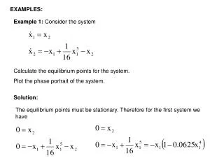
EXAMPLES: Example 1: Consider the system Calculate the equilibrium points for the system. Plot the phase portrait of the system. Solution: The equilibrium points must be stationary. Therefore for the first system we have
roots([-1/16 0 0 0 1]) ans = -2.0000 -0.0000 + 2.0000i -0.0000 - 2.0000i 2.0000 x1=0 The jacobian matrix is defined as The equilibrium points are xe=[(0,0),(2,0),(-2,0)]
The same result is obtained for xe3 (2,0) Saddle points Stable node [x1, x2] = meshgrid(-4:0.2:4, -2:0.2:2); x1dot = x2; x2dot = -x1+(1/16)*x1.^5-x2; quiver(x1,x2,x1dot,x2dot) xlabel('x_1') ylabel('x_2')
Example 2. Show that the origin of the system is stable, using a suitable Lyapunov function. Solution: Let us use the following Lyapunov function The system is stable in the sense of Lyapunov.
Example 3: R(s) + y C(s) - y3 N s Find the describing function of the nonlinear element N of the control system. For a sinusoidal input a1=0
>>syms tet;syms A; >>b1=‘((3*A^3/4)*sin(tet)-A^3/4*sin(3*tet))*sin(tet)’; >>int(b1,-pi,pi) N(A)
Example 4: R(s) + 1 -1 - Determine whether the system in the Figure exhibits a self-sustained oscillation (a limit cycle). C(s) N(A,ω) Since there is always a negative real part, the system doesn’t exhibit a limit cycle.
LYAPUNOV STABILITY FOR LINEAR TIME-INVARIANT SYSTEMS: Given a linear system of the form Let us consider a quadratic Lyapunov function candidate where P is a given symmetric positive definite matrix.
Differentiating the positive definite function V along the system trajectory yields another quadratic form where If there exists a positive definite matrix Q satisfying the equation (Lyapunov equation), the system is said to be stable in the sense of Lyapunov (ISL). Lyapunov equation.
A useful way of studying a given linear system using scalar quadratic functions is to derive a positive definite matrix P from a given positive definite matrix Q, i.e., • choose a positive definite matrix Q • solve for P from the Lyapunov equation • check whether P is positive definite If P is positive definite, then xTPx is a Lyapunov function for the linear system and global asymptotical stability is guaranteed.
Example: Consider two matrices, The linear system is stable (Real parts of all eigenvalues of the system matrix A are negative) if there is a positive definite matrix P. Using Matlab, we can find the matrix P as P = 0.4010 -0.5000 -0.5000 0.8125 ans = 0.0661 1.1474 clc;clear; A=[0 1;-12 -8]; Q=[1 0;0 1]; P=lyap(A,Q) eig(P) The matrix P is positive definite, since the eigenvalues are real, and the system is stable ISL.
LYAPUNOV FUNCTION FOR NONLINEAR SYSTEM: Krasovskii’s method suggests a simple form of Lyapunov function candidate (LFC) for autonomous nonlinear systems, namely, V=fTf. The basic idea of the method is simply to check whether this particular choice indeed leads to a Lyapunov function. Theorem (Krasovskii): Consider the autonomous system defined by dx/dt=f(x), with the equilibrium point of interest being the origin. Let J(x) denote the Jacobian matrix of the system, i.e., If the matrix F=J+JT is negative definite, the equilibrium point at the origin is asymptotically stable. A Lyapunov function for this system is If V(x) ∞ as ǁxǁ ∞, then the equilibrium point is globally asymptotically stable.
Example: Consider a nonlinear system We have
The matrix F is negative definite over the whole state space. Therefore, the origin is asymptotically stable, and a Lyapunov function candidate is clc;clear; x2=-10:0.1:10; for i=1:length(x2) F=[-12 4;4 -12-12*x2(i)^2]; eg=eig(F) plot(eg(1),eg(2)) hold on end Since V(x) ∞ as ǁxǁ ∞, then the equilibrium point is globally asymptotically stable.
Example (Variable Gradient Method): Consider a nonlinear system We assume that the gradient of the undetermined Lyapunov function has the following form The curl equation is Slotine and Li, Applied Nonlinear Control
If the coefficients are choosen to be a11=a22=1, a12=a21=0 which leads to Then Thus, dV/dt is locally negative definite in the region (1-x1x2)>0. the function V can be computed as This is indeed positive definite, and therefore the asymptotic stability is guaranteed. Slotine and Li, Applied Nonlinear Control