Download
1 / 23
230 likes | 522 Vues
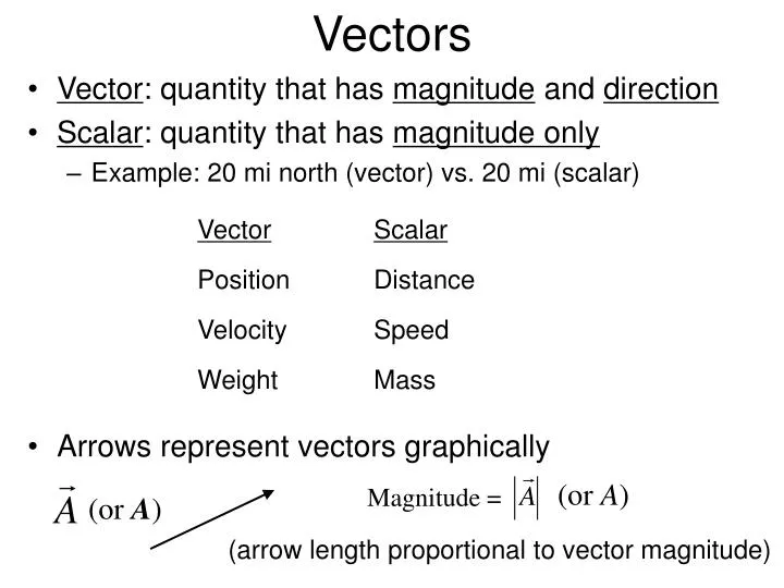
Vectors. Vector : quantity that has magnitude and direction Scalar : quantity that has magnitude only Example: 20 mi north (vector) vs. 20 mi (scalar) Arrows represent vectors graphically. (or A ). Magnitude = . (or A ). (arrow length proportional to vector magnitude). A. A. B. B.

E N D
Vectors • Vector: quantity that has magnitude and direction • Scalar: quantity that has magnitude only • Example: 20 mi north (vector) vs. 20 mi (scalar) • Arrows represent vectors graphically (or A) Magnitude = (or A) (arrow length proportional to vector magnitude)
A A B B Vectors • Two vectorsAandBare equal if|A| = |B| ANDA B: • For vectorCantiparallel toAandB, with same length asAandB A = B = – C • Vector addition: Must take direction into account! • Use tail-to-tip rule: place tail of 2nd vector to tip of 1st vector • Works for any number of vectors C
B B A A C B D E –B A–B Vector Addition and Subtraction • ForA + B = C: • Vector addition is commutative (order doesn’t matter) – try it! • For multiple vectorsA + B+ D= E: • Rules for vector subtraction are the same – just consider adding a negative vector: Vector Addition and Subtraction Interactive A A A – B= A + (– B)
Ax Ay Ay Ax Component Vectors • Imagine the hassle of measuring a triangle each time you want to add vectors! • Would need protractor, ruler, etc. • Use of vector components provides simple yet accurate method for adding vectors y Axand Ay are determined from trigonometry: Ax = Acosq and Ay = Asinq Ax(Ay) could be positive or negative depending on whether or not it points in the +x or –x (+y or –y) direction A = Ax+ Ay A q x A = (Ax2 + Ay2)1/2
x y Ay Ax Component Vectors • It may be helpful to envision components as “shadows” that are projected along each axis: • The length of the “shadow” depends on the orientation of A y A q x
Component Vectors • Any vector can be represented by its x and y component vectors • Sometimes it is convenient to determine the components of vectors in a tilted coordinate system:
In terms of components: By Ay Cy Ax Bx Cx Component Vectors y B Ax + Bx = Cx Ay + By = Cy C • Using components to add vectors A + B = C: A x
Example Problem #3.18 Solution (details given in class): (a) 185 N, q = 77.80 (above +x axis) (b) 185 N, q = 2580 (or 77.80below –x axis)
z y x 2–D and 3–D Motion • Strong similarity between 1–D motion and 2–D (or 3–D) motion • Same kinematic quantities (displacement, velocity, acceleration) are used • Only difference is vector quantities can have up to three non-zero components • First, we describe position: • Displacement (change in position):
2–D and 3–D Velocity • Average velocity: • Or: • Instantaneous velocity: • Instantaneous speed: • Think Pythagorean theorem! • Just like in 1–D motion, average velocity only depends on beginning and ending position • Instantaneous velocity is tangent to the curve of versus time
2–D and 3–D Acceleration (same as 1–D) • Average acceleration defined as: • are the instantaneous velocities at t2 and t1, respectively • points in the same direction as • Instantaneous acceleration: • points toward the inside of any turn particle is making • Remember that an object can have a non-zero acceleration even though its speed remains unchanged • Example: uniform circular motion • Speed remains the same • Velocity keeps changing due to changing direction (same as 1–D)
v0 Projectile Motion • Have you ever wondered how to predict how far a batted baseball will travel, or how far a skier will travel after jumping from a ramp? • These are examples of projectile motion • Projectile (baseball, skier) follows a trajectory (path in space) determined by its initial velocity and effects of gravity • Start with simple model • Projectile represented by single particle • Neglect air resistance, curvature & rotation of the earth y (Usually put start of motion at origin of coordinates) x
v0y v0x Projectile Motion • Notice that acceleration is constant (= g) and is in vertical direction (due to gravity) pointing toward earth’s surface • This is motion with constant acceleration in 2–D • Particle is given an initial velocity v0: • We can analyze projectile motion as: • Horizontal motion with constant velocity(ax = 0) • Vertical motion with constant acceleration (due to gravity) y ax = 0 vx = v0x = v0cosq (constant in time) ay = –g vy varies with time v0x v0y q x
Projectile Motion Animation • The equations describing the motion follow directly from our discussion of 1–D motion with constant acceleration: • Notice that we treat the x– and y–components separately y–direction (ay = –g): x–direction (ax = 0):
y = ymax x = xmax What is the maximum height reached? (or At what value of y is vy = 0?) What is the maximum range? (or What is the value of x when y = 0 [other than at the origin]?) Projectile Motion • You can answer lots of questions concerning the path the projectile takes by using these equations • Many times you need to restate the question to determine what the question is looking for y x
Example Problem #3.24 Solution (details given in class): • 3.19 s • 36.1 m/s, q = –60.10 (below +x axis)
Solution (details given in class): 25 m Example Problem #3.29
Simulation and solution details given in class Interactive Example Problem: Target Practice
Example Problem #3.59 y0 Solution (proof given in class): tanq0 = y0 / x0 x0
yB vB/A xB OB P xB/A xP/B xP/A Relative Velocity • What is the velocity of a car cruising down a highway? • The answer depends on the observer • Someone watching from the shoulder might say “55 mph” • Someone in another car traveling in same direction may say “0 mph relative to my speed” • Each observer, equipped with the proper measuring apparatus (i.e. meter stick + stopwatch), forms a frame of reference (coordinate system + time scale) • The geometry of reference frames: yA xA OA
Relative Velocity • From the figure, we see that xB/A + xP/B = xP/A • A similar relationship holds between the relative velocities: • There is a natural extension to 2 – or 3 – D motion • Relative positions are described by position vectors : • The relative velocities are given by:
Solution (details given in class): 249 ft Example Problem #3.39