Magnetic Disk Characteristics I/O Connection Structure Types of Buses Cache & I/O

Magnetic Disk Characteristics • I/O Connection Structure • Types of Buses • Cache & I/O • I/O Performance Metrics • I/O System Modeling Using Queuing Theory • Designing an I/O System • RAID (Redundant Array of Inexpensive Disks) • I/O Benchmarks • ABCs of UNIX File Systems • A Study Comparing UNIX File System Performance

RAID (Redundant Array of Inexpensive Disks) • The term RAID was coined in a 1988 paper by Patterson, Gibson and Katz of the University of California at Berkeley. • In that article, the authors proposed that large arrays of small, inexpensive disks --usually SCSI, IDE support just started-- could be used to replace the large, expensive disks used on mainframes and minicomputers. • In such arrays files are "striped" and/or mirrored across multiple drives. • Their analysis showed that the cost per megabyte could be substantially reduced, while both performance (throughput) and fault tolerance could be increased. • The Catch: Array Reliability without any redundancy : Reliability of N disks = Reliability of 1 Disk ÷ N 50,000 Hours ÷ 70 disks = 700 hours • Disk system MTTF: Drops from 6 years to 1 month! • Arrays (without redundancy) too unreliable to be useful!

Manufacturing Advantages of Disk Arrays Disk Product Families Conventional: 4 disk form factors 14” 3.5” 5.25” 10” High End Low End Disk Array: 1 disk form factor 3.5”

RAID Subsystem Organization array controller host single board disk controller host adapter manages interface to host, DMA single board disk controller control, buffering, parity logic single board disk controller physical device control single board disk controller Striping software off-loaded from host to array controller No application modifications No reduction of host performance often piggy-backed in small format devices

Basic RAID Organizations • Non-Redundant (RAID Level 0) • Mirrored (RAID Level 1) • Memory-Style ECC (RAID Level 2) • Bit-Interleaved Parity (RAID Level 3) • Block-Interleaved Parity (RAID Level 4) • Block-Interleaved Distributed-Parity (RAID Level 5) • P+Q Redundancy (RAID Level 6) • Striped Mirrors (RAID Level 10)

Non-Redundant (RAID Level 0) • RAID 0 simply stripes data across all drives (minimum 2 drives) to increase data throughput but provides no fault protection. • Sequential blocks of data are written across multiple disks in stripes, as follows: • The size of a data block, which is known as the "stripe width", varies with the implementation, but is always at least as large as a disk's sector size. • This scheme offers the best write performance since it never needs to update redundant information. • It does not have the best read performance. • Redundancy schemes that duplicate data, such as mirroring, can perform better on reads by selectively scheduling requests on the disk with the shortest expected seek and rotational delays.

Optimal Size of Data Striping Unit(Applies to RAID Levels 0, 5, 6, 10) • Lee and Katz [1991] use an analytic model of non-redundant disk arrays to derive an equation for the optimal size of data striping unit. • They show that the optimal size of data strip-ing is equal to: • Where: • P is the average disk positioning time, • X is the average disk transfer rate, • L is the concurrency, Z is the request size, and • N is the array size in disks. • Their equation also predicts that the optimal size of data striping unit is dependent only the relative rates at which a disk positions and transfers data, PX, rather than P or X individually. Lee and Katz show that the opti-mal • striping unit depends on request size; Chen and Patterson show that this dependency can be ignored without significantly affecting performance.

Mirrored (RAID Level 1) • Utilizes mirroring or shadowing of data using twice as many disks as a non-redundant disk array. • Whenever data is written to a disk the same data is also written to a redundant disk, so that there are always two copies of the information. • When data is read, it can be retrieved from the disk with the shorter queuing, seek and rotational delays • If a disk fails, the other copy is used to service requests. • Mirroring is frequently used in database applications where availability and transaction rate are more important than storage efficiency.

Memory-Style ECC (RAID Level 2) • RAID 2 performs data striping with a block size of one bit or byte, so that all disks in the array must be read to perform any read operation. • A RAID 2 system would normally have as many data disks as the word size of the computer, typically 32. • In addition, RAID 2 requires the use of extra disks to store an error-correcting code for redundancy. • With 32 data disks, a RAID 2 system would require 7 additional disks for a Hamming-code ECC. • Such an array of 39 disks was the subject of a U.S. patent granted to Unisys Corporation in 1988, but no commercial product was ever released. • For a number of reasons, including the fact that modern disk drives contain their own internal ECC, RAID 2 is not a practical disk array scheme.

Bit-Interleaved Parity (RAID Level 3) • One can improve upon memory-style ECC disk arrays ( RAID 2) by noting that, unlike memory component failures, disk controllers can easily identify which disk has failed. Thus, one can use a single parity disk rather than a set of parity disks to recover lost information. • As with RAID 2, RAID 3 must read all data disks for every read operation. • This requires synchronized disk spindles for optimal performance, and works best on a single-tasking system with large sequential data requirements. An example might be a system used to perform video editing, where huge video files must be read sequentially.

Block-Interleaved Parity (RAID Level 4) • RAID 4 is similar to RAID 3 except that blocks of data are striped across the disks rather than bits/bytes. • Read requests smaller than the striping unit access only a single data disk. • Write requests must update the requested data blocks and must also compute and update the parity block. • For large writes that touch blocks on all disks, parity is easily computed by exclusive-or’ing the new data for each disk. • For small write requests that update only one data disk, parity is computed by noting how the new data differs from the old data and apply-ing those differences to the parity block. • This can be an important performance improvement for small or random file access (like a typical database application) if the application record size can be matched to the RAID 4 block size.

Block-Interleaved Distributed-Parity (RAID Level 5) • The block-interleaved distributed-parity disk array eliminates the parity disk bottleneck present in RAID 4 by distributing the parity uniformly over all of the disks. • An additional, frequently overlooked advantage to distributing the parity is that it also distributes data over all of the disks rather than over all but one. • RAID 5 has the best small read, large read and large write performance of any redundant disk array. • Small write requests are somewhat inefficient compared with redundancy schemes such as mirroring however, due to the need to perform read-modify-write operations to update parity.

RAID-5: Small Write Algorithm 1 Logical Write = 2 Physical Reads + 2 Physical Writes D0 D1 D2 D0' D3 P old data new data old parity (1. Read) (2. Read) XOR + + XOR (3. Write) (4. Write) D0' D1 D2 D3 P' Problems of Disk Arrays: Small Writes

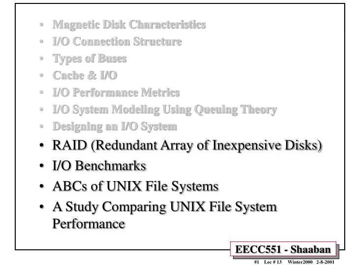
P+Q Redundancy (RAID Level 6) • An enhanced RAID 5 with stronger error-correcting codes used . • One such scheme, called P+Q redundancy, uses Reed-Solomon codes, in addition to parity, to protect against up to two disk failures using the bare minimum of two redundant disks. • The P+Q redundant disk arrays are structurally very similar to the block-interleaved distributed-parity disk arrays (RAID 5) and operate in much the same manner. • In particular, P+Q redundant disk arrays also perform small write opera-tions using a read-modify-write procedure, except that instead of four disk accesses per write requests, P+Q redundant disk arrays require six disk accesses due to the need to update both the ‘P’ and ‘Q’ information.

Increasing Logical Disk Addresses D0 D1 D2 D3 P A logical write becomes four physical I/Os Independent writes possible because of interleaved parity Reed-Solomon Codes ("Q") for protection during reconstruction D4 D5 D6 P D7 D8 D9 P D10 D11 D12 P D13 D14 D15 Stripe P D16 D17 D18 D19 Targeted for mixed applications Stripe Unit D20 D21 D22 D23 P . . . . . . . . . . . . . . . Disk Columns RAID 5/6: High I/O Rate Parity

RAID 10 (Striped Mirrors) • RAID 10 (also known as RAID 1+0) was not mentioned in the original 1988 article that defined RAID 1 through RAID 5. • The term is now used to mean the combination of RAID 0 (striping) and RAID 1 (mirroring). • Disks are mirrored in pairs for redundancy and improved performance, then data is striped across multiple disks for maximum performance. • In the diagram below, Disks 0 & 2 and Disks 1 & 3 are mirrored pairs. • Obviously, RAID 10 uses more disk space to provide redundant data than RAID 5. However, it also provides a performance advantage by reading from all disks in parallel while eliminating the write penalty of RAID 5.

RAID Levels Comparison:Throughput Per Dollar Relative to RAID Level 0.

RAID Reliability • Redundancy in disk arrays is motivated by the need to overcome disk failures. • When only independent disk failures are considered, a simple parity scheme works admirably. Patterson, Gibson, and Katz derive the mean time between failures for a RAID level 5 to be: MTTF (disk)2 / N (G - 1) MTTR(disk) • where MTTF(disk) is the mean-time-to-failure of a single disk, • MTTR(disk) is the mean-time-to-repair of a single disk, • N is the total number of disks in the disk array • G is the parity group size • For illustration purposes, let us assume we have: • 100 disks that each had a mean time to failure (MTTF) of 200,000 hours and a mean time to repair of one hour. If we organized these 100 disks into parity groups of average size 16, then the mean time to failure of the system would be an astounding 3000 years! Mean times to failure of this • magnitude lower the chances of failure over any given period of time.

Array Controller String Controller . . . String Controller . . . String Controller . . . String Controller . . . String Controller . . . String Controller . . . Data Recovery Group: unit of data redundancy System Availability: Orthogonal RAIDs Redundant Support Components: power supplies, controller, cables

System-Level Availability host host Fully dual redundant I/O Controller I/O Controller Array Controller Array Controller . . . . . . . . . Goal: No Single Points of Failure . . . . . . . . . with duplicated paths, higher performance can be obtained when there are no failures Recovery Group

I/O Benchmarks • Processor benchmarks classically aimed at response time for fixed sized problem. • I/O benchmarks typically measure throughput, possibly with upper limit on response times (or 90% of response times) • Traditional I/O benchmarks fix the problem size in the benchmark. • Examples: Benchmark Size of Data % Time I/O Year I/OStones 1 MB 26% 1990 Andrew 4.5 MB 4% 1988 • Not much I/O time in benchmarks • Limited problem size • Not measuring disk (or even main memory)

The Ideal I/O Benchmark • An I/O benchmark should help system designers and users understand why the system performs as it does. • The performance of an I/O benchmark should be limited by the I/O devices. to maintain the focus of measuring and understanding I/O systems. • The ideal I/O benchmark should scale gracefully over a wide range of current and future machines, otherwise I/O benchmarks quickly become obsolete as machines evolve. • A good I/O benchmark should allow fair comparisons across machines. • The ideal I/O benchmark would be relevant to a wide range of applications. • In order for results to be meaningful, benchmarks must be tightly specified. Results should be reproducible by general users; optimizations which are allowed and disallowed must be explicitly stated.

I/O Benchmarks Comparison

Self-scalingI/O Benchmarks • Alternative to traditional I/O benchmarks: self-scaling I/O benchmarks; automatically and dynamically increase aspects of workload to match characteristics of system measured • Measures wide range of current & future applications • Types of self-scaling benchmarks: • Transaction Processing - Interested in IOPS not bandwidth • TPC-A, TPC-B, TPC-C • NFS: SPEC SFS/ LADDIS - average response time and throughput. • Unix I/O - Performance of files systems • Willy

I/O Benchmarks: Transaction Processing • Transaction Processing (TP) (or On-line TP=OLTP) • Changes to a large body of shared information from many terminals, with the TP system guaranteeing proper behavior on a failure • If a bank’s computer fails when a customer withdraws money, the TP system would guarantee that the account is debited if the customer received the money and that the account is unchanged if the money was not received • Airline reservation systems & banks use TP • Atomic transactions makes this work • Each transaction => 2 to 10 disk I/Os & 5,000 and 20,000 CPU instructions per disk I/O • Efficiency of TP SW & avoiding disks accesses by keeping information in main memory • Classic metric is Transactions Per Second (TPS) • Under what workload? how machine configured?

I/O Benchmarks: TPC-C Complex OLTP • Models a wholesale supplier managing orders. • Order-entry conceptual model for benchmark. • Workload = 5 transaction types. • Users and database scale linearly with throughput. • Defines full-screen end-user interface • Metrics: new-order rate (tpmC) and price/performance ($/tpmC) • Approved July 1992

SPEC SFS/LADDIS Predecessor: NFSstones • NFSStones: synthetic benchmark that generates series of NFS requests from single client to test server: reads, writes, & commands & file sizes from other studies. • Problem: 1 client could not always stress server. • Files and block sizes not realistic. • Clients had to run SunOS.

SPEC SFS/LADDIS • 1993 Attempt by NFS companies to agree on standard benchmark: Legato, Auspex, Data General, DEC, Interphase, Sun. • Like NFSstones but: • Run on multiple clients & networks (to prevent bottlenecks) • Same caching policy in all clients • Reads: 85% full block & 15% partial blocks • Writes: 50% full block & 50% partial blocks • Average response time: 50 ms • Scaling: for every 100 NFS ops/sec, increase capacity 1GB. • Results: plot of server load (throughput) vs. response time & number of users • Assumes: 1 user => 10 NFS ops/sec

Unix I/O Benchmarks: Willy • UNIX File System Benchmark that gives insight into I/O system behavior (Chen and Patterson, 1993) • Self scaling to automatically explore system size • Examines five parameters • Unique bytes touched: data size; locality via LRU • Gives file cache size • Percentage of reads: %writes = 1 – % reads; typically 50% • 100% reads gives peak throughput • Average I/O Request Size: Bernoulli, C=1 • Percentage sequential requests: typically 50% • Number of processes: concurrency of workload (number processes issuing I/O requests) • Fix four parameters while vary one parameter • Searches space to find high throughput

OS Policies and I/O Performance • Performance potential determined by HW: CPU, Disk, bus, memory system. • Operating system policies can determine how much of that potential is achieved. • OS Policies: 1) How much main memory allocated for file cache? 2) Can boundary change dynamically? 3) Write policy for disk cache. • Write Through with Write Buffer • Write Back

ABCs of UNIX File Systems • Key Issues • File vs. Raw I/O • File Cache Size Policy • Write Policy • Local Disk vs. Server Disk • File vs. Raw: • File system access is the norm: standard policies apply • Raw: alternate I/O system to avoid file system, used by data bases • File Cache Size Policy • Files are cached in main memory, rather than being accessed from disk • With older UNIX, % of main memory dedicated to file cache is fixed at system generation (e.g., 10%) • With new UNIX % of main memory for file cache varies depending on amount of file I/O (e.g., up to 80%)

ABCs of UNIX File Systems • Write Policy • File Storage should be permanent; either write immediately or flush file cache after fixed period (e.g., 30 seconds) • Write Through with Write Buffer • Write Back • Write Buffer often confused with Write Back • Write Through with Write Buffer, all writes go to disk • Write Through with Write Buffer, writes are asynchronous, so processor doesn’t have to wait for disk write • Write Back will combine multiple writes to same page; hence can be called Write Cancelling

ABCs of UNIX File Systems • Local vs. Server • Unix File systems have historically had different policies (and even file systems) for local client vs. remote server • NFS local disk allows 30 second delay to flush writes • NFS server disk writes through to disk on file close • Cache coherency problem if allow are allowed to have file caches in addition to server file cache • NFS just writes through on file closeStateless protocol: periodically get new copies of file blocks • Other file systems use cache coherency with write back to check state and selectively invalidate or update

remote accesses local accesses Network File Systems

UNIX File System Performance Study Using Willy 9 Machines & OSs Machine OS Year Price Memory Alpha AXP 3000/400 OSF/1 1993 $30,000 64 MB DECstation 5000/200 Sprite LFS 1990 $20,000 32 MB DECstation 5000/200 Ultrix 4.2 1990 $20,000 32 MB HP 730 HP/UX 8 & 9 1991 $35,000 64 MB IBM RS/6000/550 AIX 3.1.5 1991 $30,000 64 MB SparcStation 1+ SunOS 4.1 1989 $30,000 28 MB SparcStation 10/30 Solaris 2.1 1992 $20,000 128 MB Convex C2/240 Convex OS 1988 $750,0001024 MB IBM 3090/600J VF AIX/ESA 1990 $1,000,000 128 MB Desktop Mini/Mainframe

Self-Scaling Benchmark Parameters

Disk Performance • 32 KB reads • SS 10 disk spins 5400 RPM; 4 IPI disks on Convex

File Cache Performance • UNIX File System Performance: not how fast disk, but whetherdisk is used (File cache has 3 to 7 x disk perf.) • 4X speedup between generations; DEC & Sparc Fast Mem Sys DEC Generations Sun Generations

File Cache Size • HP v8 (8%) vs. v9 (81%); DS 5000 Ultrix (10%) vs. Sprite (63%)

File System Write Policies • Write Through with Write Buffer (Asynchronous): AIX, Convex, OSF/1 w.t., Solaris, Ultrix Fast File Caches for Reads Fast Disks MB/sec

File cache performance vs. read percentage

Performance vs. Megabytes Touched

Write policy Performance For Client/Server Computing • NFS: write through on close (no buffers) • HPUX: client caches writes; 25X faster @ 80% reads FDDI Network MB/sec Ethernet

UNIX I/O Performance Study Conclusions • Study uses Willy, an I/O benchmark which supports self-scaling evaluation and predicted performance. • The hardware determines the potential I/O performance, but the operating system determines how much of that potential is delivered: differences of factors of 100. • File cache performance in workstations is improving rapidly, with over four-fold improvements in three years for DEC (AXP/3000 vs. DECStation 5000) and Sun (SPARCStation 10 vs. SPARCStation 1+). • File cache performance of Unix on mainframes and mini-supercomputers is no better than on workstations. • Workstations benchmarked can take advantage of high performance disks. • RAID systems can deliver much higher disk performance. • File caching policy determines performance of most I/O events, and hence is the place to start when trying to improve OS I/O performance.

Magnetic Disk Characteristics I/O Connection Structure Types of Buses Cache & I/O