Download
1 / 41
730 likes | 1.41k Vues
Solution of Linear Systems of Equations Consistency Rank Geometric Interpretation. Rank of matrix. Equal to the dimension of the largest square sub-matrix of A that has a non-zero determinant. Example:. has rank 3. Rank of matrix (cont’d).

E N D
Solution of Linear Systems of Equations • Consistency • Rank • Geometric Interpretation
Rank of matrix Equal to the dimension of the largest square sub-matrix of A that has a non-zero determinant. Example: has rank 3
Rank of matrix (cont’d) • Alternative definition: the maximum number of linearly independent columns (or rows) of A. Therefore, rank is not 4 ! Example:
Solution of Linear Systems Each side of the equation (2) Can be multiplied by A-1 : Due to the definition of A-1: Therefore the solution of (2) is:
Consistency (Solvability) • A-1 does not exist for every A • The linear system of equations A·x=b has a solution, or said to be consistent IFF Rank{A}=Rank{A|b} • A system is inconsistent when Rank{A}<Rank{A|b} Rank{A} is the maximum number of linearly independent columns or rows of A. Rank can be found by using ERO (Elementary Row Oparations) or ECO (Elementary column operations).
Elementary row and column operations • The following operations applied to the augmented matrix [A|b], yield an equivalent linear system • Interchanges: The order of two rows/columns can be changed • Scaling: Multiplying a row/column by a nonzero constant • Sum: The row can be replaced by the sum of that row and a nonzero multiple of any other row. One can use ERO and ECO to find the Rank as follows: EROminimum # of rows with at least one nonzero entry or ECOminimum # of columns with at least one nonzero entry
An inconsistent example: Geometric interpretation ERO:Multiply the first row with -2 and add to the second row Rank{A}=1 Rank{A|b}=2 > Rank{A}
Uniqueness of solutions • The system has a unique solution IFF Rank{A}=Rank{A|b}=n n is the order of the system • Such systems are called full-rank systems
Full-rank systems • If Rank{A}=n Det{A} 0 A-1 exists Unique solution
Rank deficient matrices • If Rank{A}=m<n Det{A} = 0 A is singular so not invertible infinite number of solutions (n-m free variables) under-determined system Rank{A}=Rank{A|b}=1 Consistent so solvable
Ill-conditioned system of equations • A small deviation in the entries of A matrix, causes a large deviation in the solution.
Ill-conditioned continued..... A linear system of equations is said to be “ill-conditioned” if the coefficient matrix tends to be singular
Back substitution ERO Gaussian Elimination • By using ERO, matrix A is transformed into an upper triangular matrix (all elements below diagonal 0) • Back substitution is used to solve the upper-triangular system
Ill-Conditioned Matrices • Matrix inversion: Ax = b x = A-1b • Assume A is a perfectly known matrix • Consider b to be obtained from measurement with some uncertainty • Terminology • Well-conditioned problem: “small” changes in the data b produce “small” changes in the solution x • Ill-conditioned problem: “small” changes in the data b produce “large” changes in the solution x • Ill-conditioned matrices • Caused by nearly linearly dependent equations • Characterized by nearly singular A matrix • Solution is not reliable • Common problem for large algebraic systems • Ill-conditioning quantified by the condition number (covered later)
Ill-Conditioned Matrix Example • Example • e represents measurement error in b2 • Two rows (columns) are nearly linearly dependent • Analytical solution • 10% error (e = 0.1)
Definitions Definition 1: A nonzero vector x is an eigenvector (or characteristic vector) of a square matrix A if there exists a scalar λ such that Ax = λx. Then λ is an eigenvalue (or characteristic value) of A. Note: The zero vector can not be an eigenvector even though A0 = λ0. But λ = 0 can be an eigenvalue. Example:
Geometric interpretation of Eigenvalues and Eigenvectors An n×n matrix A multiplied by n×1 vector x results in another n×1 vector y=Ax. Thus A can be considered as a transformation matrix. In general, a matrix acts on a vector by changing both its magnitude and its direction. However, a matrix may act on certain vectors by changing only their magnitude, and leaving their direction unchanged (or possibly reversing it). These vectors are the eigenvectors of the matrix. A matrix acts on an eigenvector by multiplying its magnitude by a factor, which is positive if its direction is unchanged and negative if its direction is reversed. This factor is the eigenvalue associated with that eigenvector.
Eigenvalues Let x be an eigenvector of the matrix A. Then there must exist an eigenvalue λ such that Ax = λx or, equivalently, Ax - λx= 0 or (A – λI)x= 0 If we define a new matrix B = A – λI, then Bx= 0 If B has an inverse then x = B-10 = 0. But an eigenvector cannot be zero. Thus, it follows that x will be an eigenvector of A if and only if B does not have an inverse, or equivalently det(B)=0, or det(A – λI)= 0 This is called the characteristic equation of A. Its roots determine the eigenvalues of A.
Eigenvalues: examples Example 1: Find the eigenvalues of two eigenvalues: 1, 2 Note: The roots of the characteristic equation can be repeated. That is, λ1 = λ2 =…= λk. If that happens, the eigenvalue is said to be of multiplicity k. Example 2: Find the eigenvalues of λ = 2 is an eigenvector of multiplicity 3.
Eigenvectors To each distinct eigenvalue of a matrix A there will correspond at least one eigenvector which can be found by solving the appropriate set of homogenous equations. If λi is an eigenvalue then the corresponding eigenvector xi is the solution of (A – λiI)xi= 0 Example 1 (cont.):
Eigenvectors Example 2 (cont.): Find the eigenvectors of Recall that λ = 2 is an eigenvector of multiplicity 3. Solve the homogeneous linear system represented by Let . The eigenvectors of = 2 are of the form s and t not both zero.
Properties of Eigenvalues and Eigenvectors Definition: The trace of a matrix A, designated by tr(A), is the sum of the elements on the main diagonal. Property 1: The sum of the eigenvalues of a matrix equals the trace of the matrix. Property 2: A matrix is singular if and only if it has a zero eigenvalue. Property 3: The eigenvalues of an upper (or lower) triangular matrix are the elements on the main diagonal. Property 4: If λ is an eigenvalue of A and A is invertible, then 1/λ is an eigenvalue of matrix A-1.
Properties of Eigenvalues and Eigenvectors Property 5: If λ is an eigenvalue of A then kλ is an eigenvalue of kA where k is any arbitrary scalar. Property 6: If λ is an eigenvalue of A then λk is an eigenvalue of Ak for any positive integer k. Property 8: If λ is an eigenvalue of A then λ is an eigenvalue of AT. Property 9: The product of the eigenvalues (counting multiplicity) of a matrix equals the determinant of the matrix.
Linearly independent eigenvectors Theorem: Eigenvectors corresponding to distinct (that is, different) eigenvalues are linearly independent. Theorem: If λ is an eigenvalue of multiplicity k of an nn matrix A then the number of linearly independent eigenvectors of A associated with λ is given by m = n - r(A- λI). Furthermore, 1 ≤ m ≤ k. Example 2 (cont.): The eigenvectors of = 2 are of the form s and t not both zero. = 2 has two linearly independent eigenvectors
Cayley Hamilton Theorem Statement : Every square matrix satisfies its characteristic equation. Possible Questions based on Cayley-Hamilton theorem 1. Find Characteristic Equation of a matrix. 2. Verify Cayley-Hamilton theorem . 3. Find the inverse of a matrix. 4. Find the matrix represented by polynomial of a matrix
Find the characteristic equation of the matrix Show that the equation is satisfied by A. Also find A-1 . Using Cayley - Hamilton theorem, find If
Thm : Eigen values of a Unitary matrix are of unit modulus Proof: Let ‘A’ be a Unitary matrix, so .…. (1) and ‘𝜆’ is eigen value of ‘A’ , then A X = 𝜆 X ……(2) Taking transposed conjugate in eqn. (2) …(3)
Cryptography Cryptography is concerned with keeping communications private.
Cryptography consists of Encryption (encoding) and Decryption (decoding) Cryptography makes use of a matrix to encode a message. The receiver of the message decodes it using the inverse of the matrix. The matrix, used by the sender is called the encoding matrix and its inverse is called the decoding matrix, which is used by the receiver.
Matrix inverses can provide a simple and effective procedure for encoding and decoding messages. To begin, assign the numbers 1-26 to the letters in the alphabet, as shown below. Also assign the number 0 to a blank to provide for space between words. Blank A B C D E F G H I J K L M N O P Q R S T U V W X Y Z 0 1 2 3 4 5 6 7 8 9 10 11 12 13 14 15 16 17 18 19 20 21 22 23 24 25 26
Steps to create a cryptogram To encode “MY NAME IS RAJ”, Write the sequence as 13, 25, 0, 14, 1, 13, 5, 0, 9, 19, 0, 18, 1, 10, 0 and the Message matrix can be written as M =
Steps to ENCODE MESSAGES To encode a message, choose a 3x3 matrix A that has an inverse and multiply ‘A’ on the left with matrix ‘M’ Let A = , So the encrypted matrix, X = A . M = . =
Decoding using Matrix INVERSE Find the inverse of ‘A’, Since X = A.M, so M = . X = The receiver obtain the sequence of numbers as 13, 25, 0, 14, 1, 13, 5, 0, 9, 19, 0, 18, 1, 10, 0 The message can be retrieved with reference to the table of letters as ‘MY-NAME-IS-RAJ’