W. A. Curtin A. Needleman, C. Briant, S. Kumar, H. Kumar, J. Arata, W. Xuan

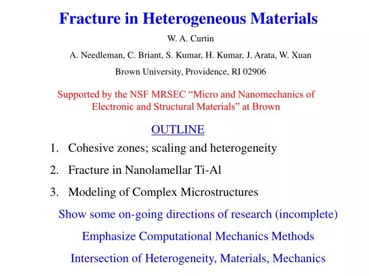
1. Fracture in Heterogeneous Materials W. A. Curtin A. Needleman, C. Briant, S. Kumar, H. Kumar, J. Arata, W. Xuan Brown University, Providence, RI 02906 Supported by the NSF MRSEC “Micro and Nanomechanics of Electronic and Structural Materials” at Brown OUTLINE • Cohesive zones; scaling and heterogeneity • Fracture in Nanolamellar Ti-Al • Modeling of Complex Microstructures • Show some on-going directions of research (incomplete) • Emphasize Computational Mechanics Methods • Intersection of Heterogeneity, Materials, Mechanics

2. Maximum stress , followed by softening Material separates naturally Nucleation without pre-existing cracks= inherent strength of material T Work of Separation = Energy to create new surface contains all energy/dissipation physically occuring within material Cohesive Zone Model: Replace localized non-linear deformation zone by an equivalent set of tractions that this material exerts on the surrounding elastic material u Cohesive Zone Model (CZM) contains several key features: (follows from work/energy arguments, e.g. J-integral)

3. If uc << all other lengths in problem: “small scale yielding”: stress intensity is a useful fracture parameter fracture is governed by critical Kc or details of T vs. u are irrelevant, only is important u* If uc ~ other lengths in problem: “large-scale bridging”: fracture behavior is geometry and scale-dependent uc If uc >> all other lengths in problem: fracture controlled by Scaling: Cohesive Zone Model introduces a LENGTH uc E=Elastic modulus of bulk material uc= Characteristic Length of Cohesive Zone at Failure Scale of heterogeneity vs. Scale of decohesion is important

4. Increasing H concentration Form T vs. u specific to physics and mechanics of decohesion: Polymer crazing: “Dugdale Model” Fiber bridging: “Sliding/Pullout Model” Polymer craze material drawn out of bulk at ~ constant stress Fiber/matrix interface sliding friction, fiber fracture, pullout Atomistic separation: “Universal Binding” First-Principles Quantum Calculations: u

5. Cracks form at cohesive strength ; difficult to stop Distributed, Nucleated Damage: difficult to model in brittle systems Imagine local stress concentration that nucleates crack; will crack stop if it encounters a region of higher toughness? uc Stress concentration is huge or Length scale of heterogeneity is small Crack stops if: Can’t stop “typical” nucleated crack in brittle materials

6. Multiscale Modeling of Fracture in Ti-Al: Microcracks Ti3Al “Colonies” of lamellae 500 microns Ti-Al: Alternating nanoscale layers of TiAl and Ti3Al Toughening: Occurs at Colony Boundaries 1 microns Fracture in Ti-Al: preferentially along lamellar direction

7. How much toughening due to boundary misorientation? Does microcracking enhance toughness? Microcracking at scales >> lamellar spacing Why? Where are cracks: TiAl, Ti3Al, or at TiAl/Ti3Al interface? Does small-scale fracture toughness depend on lamellar structure? Questions to answer about real material: Role of microstructure and heterogeneity at various scales Modeling across scales to address issues, guide optimal material design

8. Multiscale Modeling of Ti-Al: Cohesive Zones reflecting varying TiAl widths 1 Atomistics of fracture in nanolamellar Ti-Al Realistic models of colony boundary damage Toughness vs. TiAl Lamellar Thickness (Cohesive Zones) 10 um Continuum models Analytic selection of likely planes for microcracking Model of realistic colony microstructure Prediction of damage evolution, toughening vs. microstructure

9. Atomistic Simulations: Derive Toughness vs. Nanolamellar Structure Crack growth in TiAl lamella between two Ti3Al lamellae: Dislocation emission followed by crack cleavage; depends on microstructure

10. 60 nm 50 nm 40 nm 30 nm Fracture toughness increases with increasing lamellar thickness Applied KI vs. Crack Growth (R-curve): : linear scaling Fracture/Dislocation Model predicts this behavior: Toughness: Scales with square root of lamellar thickness; Thicker is tougher

11. Fracture strongly preferred along lamellar direction Thin TiAl lamellae are “weak link” in Ti-Al nanolaminates Cracks inhibited at “colony” boundaries preferentially • renucleate across boundary in thinTiAl layers • microcrack in thinTiAl layers Implications for fracture in Ti-Al nanolaminates: thinTiAl

12. Low-toughness planes Initial Crack Heterogeneous Toughnesses Mesoscale Model of Fracture Across Colony Boundaries Model of lamellar colony boundary: “Real” microstructure Computational microstructure: • Lamellar misorientation • Low-toughness lamellae modeled by cohesive zones • Heterogeneity in toughness due to variations in lamellar thickness • 1 um low-toughness lamellar spacing • Elastic matrix w/ fracture via cohesive zones Where, when do cracks nucleate? Interplay of heterogeneity, length scales?

13. 2.03.04.03.02.01.5 1.0 1.0 2.02.53.5 2.51.52.01.5 1.0 1.52.53.5 1.5 2.01.51.0 1 um Microcrack on weak plane away from main crack Microcrack on weak plane near main crack Two microcracks on weak planes away from main crack Numerical Results on Fracture in Heterogeneous Lamellar System: Impose range of low-toughness values; explore microcrack nucleation Heterogeneity can drive distributed microcracking Microcrack Nucleation: critical stress needed over some distance

14. Microstructural Model for Fracture in Ti-Al: Scale of weak planes set by heterogeneity, not lamellar scale (real microstructural-specific models not included yet) “Real” microstructure Computational microstructure: • Lamellar misorientation • Colony boundary layer modeled by cohesive zones • Low-toughness lamellae modeled by cohesive zones • 20 um low-toughness lamellar spacing: weakest lamellae • Elastic/plastic matrix w/ fracture via cohesive zones

15. Toughening as crack crosses colony boundaries Fracture through Polycolony Lamellar Ti-Al:

16. Multiple microcracking Only slight decrease in toughening Experiment Modified Colony 5 Orientation: Orientation highly unfavorable for cracking

17. Decrease in Matrix Yield Stress  More damage, higher toughness Microcrack closure (reversible cohesive zone)

18. Microstructural models capture range of physical phenomena Subtle interplay between toughnesses of various phases and boundaries, and plastic behavior Small changes in microscopic quantitities can lead to large changes in macroscopic modes of cracking and toughening Optimization of material for engineering requires understanding of Microscopic Details (alloying to harden/strengthen) Control of Microstructure (colony size, distribution)

19. Summary for Ti-Al • Cohesive Zone Model: powerful technique for nucleation and crack growth naturally: derive from smaller-scale input • Ti-Al: Nano/micro scale structure determines lamellar toughness • CZMs shows heterogeneity in microstructure at sub-micron scale can drive microcracking on larger scales • CZMs at microstructural scale capture physical phenomena, competition between toughness, plasticity, microstructure • Coupled Multiscale Models may guide optimization of microstructures for mechanical performance • 3d Fracture is important: extend CZ and Microstructure models

20. Modeling of Complex Microstructures • Experimental optimization of microstructures could be guided by insight from computations • Failure behavior is controlled by undesirable features; computations could identify such features - what should experimentalists look for? help avoid unexpected failure? • Generate a family of microstructures “statistically similar” to a real system • Computationally test microstructures • Probe dependence of performance on microstructure • Investigate optimum classes of microstructures • Compare simulated performance to experimental results • Guide fabrication toward optimal microstructures Goal: Identify global and local microstructural correlation functions that influence flow, hardening, failure; Use knowledge to guide experimental microstructural design

21. 1. Digitized microstructure of “parent”; label each pixel by phase; Calculate P2(r) and L2(r)by scanning along horizontal, vertical lines Initial Digitized 2. Generate initial reconstructed microstructure; Fix volume fraction = parent value; Compute the P2(r) and L2(r) (Yeong + Torquato) Microstructure Reconstruction: 3. Calculate the “energy” E (mean square difference) between parent, synthetic microstructure. 4. Evolve E through Simulated Annealing: Consider exchange of two sites Compute energy change Accept exchange with probability P T=“temperature”: decrease by ad-hoc annealing schedule.

22. Sample Evolution Path Initial After 45 steps After 60 steps Parent Final

23. Key Features of Reconstruction Method: • Simple to implement for arbitrary systems • Unbiased treatment of microstructures • Can incorporate a variety of correlation functions (limited only by simulated annealing time) • 3d structures can be generated using correlation functions obtained from 2d images • Multiple realizations of the same parent microstructure can be generated and tested • Microstructures already naturally in a form suitable for numerical computations via FEM (pixel = element) • Can construct NEW structures from hypothetical correlation functions • Microstructures can be built around “defects” or “hot spots” of interest to probe them

24. 2D image of Parent microstructure Cut Along the xz-plane Cut Along the yz-plane Cut Along the xy-plane

25. Real, Complex Microstructures: Ductile Iron Correlation Functions P2 Child #1 Parent Child #2 L2 Carbon Iron Child #3

26. E (GPa) Fe matrix 210 0.30 C particles 15 0.26 Finite Element Analysis: Elastic/Plastic Matrix Uniaxial Tension Stress-Strain Response Parent, Children essentially identical ! Microstructure-induced Hardening Matrix only Low-order correlations: excellent description of non-linear response What microstructural features trigger LOCALIZATION?

27. Local Onset of Instability: Sample-to-Sample Variations (of course) Parent Child #1 Child #2 Child #3 Onset U=0.150; s=847 MPa U=0.141; s=856 MPa U=0.118; s=829 MPa U=0.109; s=808 MPa Instability U=0.200; s=855 MPa U=0.234; s=857 MPa U=0.207; s=858 MPa U=0.204; s=855 MPa What is characteristic “weak” feature driving localization?

28. “Genetic” Methodology for Identification of Hot Spots: Identify hot spot; Choose test box Extract test box microstructure Build new microstructures around box Insert into new reconstruction (Grandchild) Test new microstructuresAnalyze hot spot behaviorVary test box size and retest

29. Analyze worst of the children (statistical tail): Window = 15 X 15 Grandchild Strain=15.10% Stress=847MPa Strain=19.59 % Stress=855MPa Onset mostly at another location, much higher stress and strain range Window = 20 X 20 Grandchild Strain = 25.00 % Stress = 856 MPa Strain = 11.60 % Stress = 795 MPa Onset often at same location, same stress and strain range

30. Window = 30 X 30 Grandchild Strain = 11.90 % Stress= 798 MPa Strain = 20.15 % Stress= 855 MPa Onset mostly at same location, similar stress and strain Computational identification of “characteristic” weak-link microstructure

31. Quantitative Evaluation of Hot Spot Damage Nucleation 15 x 15 Not similar to Child 20 x 20 Often similar to Child 30 x 30 Mostly similar to Child 847 15.16 Characteristic size & structure consistently drives low-stress localization event

32. Summary • “Reconstruction” Methodology • Method can establish sizes for statistical similarity (representative volume elements) • Method can identify, represent anisotropy • Current method has difficulty with isotropic, elongated structures • Examples demonstrated • Stress-strain behavior controlled by low-order structural correlations! • Localization is microstructure-specific (not surprising) • Quantitatively analyze hot spots driving failure • Successive generations allow weak-links to be isolated • Example calculations show characteristic hot-spot size

33. Future Work • Further pursue 3-d reconstruction algorithm • Cohesive zones for fracture initiation, propagation • Extend hot-spot analysis methods statistical characterization? • Validate model quantitatively vs. experiments • Methods for optimization? • Hard work still ahead ……