Download
1 / 34
340 likes | 437 Vues
The Structure of the Proton. Parton Model QCD as the theory of strong interactions Parton Distribution Functions Extending QCD calculations across the kinematic plane – understanding small-x, high density, non-perturbative regions. A.M.Cooper-Sarkar Feb 6 th 2003 RSE.

E N D
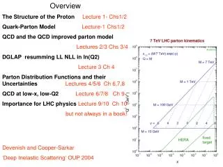
The Structure of the Proton • Parton Model • QCD as the theory of strong interactions • Parton Distribution Functions • Extending QCD calculations across the kinematic plane – understanding small-x, high density, non-perturbative regions A.M.Cooper-Sarkar Feb 6th 2003 RSE
Leptonic tensor - calculable 2 LmnWmn dF~ Hadronic tensor- constrained by Lorentz invariance Et q = k – k,Q2 = -q2 Px = p + q , W2 = (p + q)2 s= (p + k)2 x = Q2 / (2p.q) y = (p.q)/(p.k) W2 = Q2 (1/x – 1) Q2 = s x y Ee Ep s = 4 Ee Ep Q2 = 4 Ee Esin2e/2 y = (1 – E/Ee cos2e/2) x = Q2/sy The kinematic variables are measurable
d2s(e±N) = [ Y+ F2(x,Q2) - y2 FL(x,Q2) K Y_xF3(x,Q2)], YK = 1 K (1-y)2 dxdy for charged lepton hadron scattering F2, FL and xF3 are structure functions – The Quark Parton Model interprets them ds = 2pa2ei2 xs [ 1 + (1-y)2] , for elastic eq dy Q4 d2s= 2pa2 s [ 1 + (1-y)2] Giei2(xq(x) + xq(x)) dxdy Q4 for eN non-isotropic isotropic (xP+q)2=x2p2+q2+2xp.q ~ 0 for massless quarks and p2~0so x = Q2/(2p.q) The FRACTIONAL momentum of the incoming nucleon taken by the struck quark is the MEASURABLE quantity x Now compare the general equation to the QPM prediction F2(x,Q2) = Giei2(xq(x) + xq(x)) – Bjorken scaling FL(x,Q2) = 0 - spin ½ quarks xF3(x,Q2) = 0 - only ( exchange
Consider n,n scattering: neutrinos are handed ds(n)= GF2 x s ds(n) = GF2 x s (1-y)2 Compare to the general form of the cross-section for n/n scattering via W+/- FL(x,Q2) = 0 xF3(x,Q2) = 2Gix(qi(x) - qi(x)) Valence F2(x,Q2) = 2Gix(qi(x) + qi(x)) Valence and Sea And there will be a relationship between F2eN and F2nN NOTE n,n scattering is FLAVOUR sensitive dy p dy p For nq (left-left) For n q (left-right) d2s(n) = GF2 s Gi [xqi(x) +(1-y)2xqi(x)] dxdy p For nN d2s(n) = GF2 s Gi [xqi(x) +(1-y)2xqi(x)] dxdy p For nN Clearly there are antiquarks in the nucleon 3 Valence quarks plus a flavourless qq Sea m- W+ can only hit quarks of charge -e/3 or antiquarks -2e/3 n W+ u d s(np)~ (d + s) + (1- y)2 (u + c) s(np) ~ (u + c) (1- y)2 + (d + s) q = qvalence +qsea q = qsea qsea= qsea
So in n,n scattering the sums over q, q ONLY contain the appropriate flavours BUT- high statistics n,n data are taken on isoscalar targets e.g. Fe Y (p + n)/2=N d in proton = u in neutron u in proton = d in neutron GLS sum rule Total momentum of quarks A TRIUMPH (and 20 years of understanding the c c contribution)
QCD improves the Quark Parton Model I F2(<N) dx ~ 0.5 where did the momentum go? What if or x x Pqq Pgq y y Before the quark is struck? Pqg Pgg y > x, z = x/y Note q(x,Q2) ~ s lnQ2, but s(Q2)~1/lnQ2, so s lnQ2 is O(1), so we must sum all terms sn lnQ2n Leading Log Approximation x decreases from s s(Q2) xi+1 xi xi-1 target to probe xi-1> xi > xi+1…. pt2 of quark relative to proton increases from target to probe pt2i-1 < pt2i < pt2i+1 Dominant diagrams have STRONG pt ordering The DGLAP equations
Bjorken scaling is broken – ln(Q2) Note strong rise at small x Terrific expansion in measured range across the x, Q2 plane throughout the 90’s HERA data Pre HERA fixed target mp,mD NMC,BDCMS, E665 and n,n Fe CCFR
Valence distributions evolve slowly • Sea/Gluon distributions evolve fast • Parton Distribution Functions PDFs are extracted by MRST, CTEQ, ZEUS, H1 • Parametrise the PDFs at Q20 (low-scale) Note scale of xg, xS • xuv(x) =Auxau (1-x)bu (1+ eu√x + gu x) • xdv(x) =Adxad (1-x)bd (1+ ed√x + gdx) • xS(x) =Asx-ls (1-x)bs (1+ es√x + gsx) • xg(x) =Agx-lg(1-x)bg (1+ eg√x + ggx) • Some parameters are fixed through sum rules- • others by model choices- typically ~15 parameters • Use QCD to evolve these PDFs to Q2 > Q20 • Construct the measurable structure functions in terms of PDFs for ~1500 data points across the x,Q2 plane • Perform c2 fit Note error bands on PDFs
The fact that so few parameters allows us to fit so many data points established QCD as the THEORY OF THE STRONG INTERACTION and provided the first measurements of s (as one of the fit parameters) • These days we assume the validity of the picture to measure PDFs which are transportable to other hadronic processes • But where is the information coming from? • F2(e/mp)~ 4/9 x(u +u) +1/9x(d+d) • F2(e/mD)~5/18 x(u+u+d+d) • u is dominant , valence dv, uv only accessible at high x • (d and u in the sea are NOT equal, dv/uv Y 0 as x Y 1) • Valence information at small x only from xF3(nFe) • xF3(nN) = x(uv + dv) - BUT Beware Fe target! • HERA data is just ep: xS, xg at small x • xS directly from F2 • xg indirectly from scaling violations dF2 /dlnQ2 Fixed target :p/D data- Valence and Sea
HERA at high Q2Y Z0 and W+/- become as important as • exchange Y NC and CC cross-sections comparable for NC processes F2= 3i Ai(Q2) [xqi(x,Q2) + xqi(x,Q2)] xF3= 3iBi(Q2) [xqi(x,Q2) - xqi(x,Q2)] Ai(Q2) = ei2 – 2 eivi vePZ + (ve2+ae2)(vi2+ai2) PZ2 Bi(Q2) = – 2 eiai ae PZ + 4ai ae vi ve PZ2 PZ2 = Q2/(Q2 + M2Z) 1/sin2W • a new valence structure function xF3 measurable from low to high x- on a pure proton target Y sensitivity to sin2W, MZ and electroweak couplingsvi,ai for u and d type quarks- (with electron beam polarization)
CC processes give flavour information d2s(e+p) = GF2 M4W [x (u+c) + (1-y)2x (d+s)] d2s(e-p) = GF2 M4W [x (u+c) + (1-y)2x (d+s)] dxdy 2px(Q2+M2W)2 dxdy 2px(Q2+M2W)2 uv at high x dv at high x MW information Measurement of high x dvon a pure proton target (even Deuterium needs corrections, does dv/uvY 0, as x Y 1? )
Valence PDFs from ZEUS data alone- NC and CC e+ and e- beams Y high x valence dv from CC e+, uv from CC e- and NC e+/- Valence PDFs from a GLOBAL fit to all DIS data Y high x valence from CCFR xF3(n,nFe) data and NMC F2(mp)/F2(mD) ratio
Parton distributions are transportable to other processes Accurate knowledge of them is essential for calculations of cross-sections of any process involving hadrons. Conversely, some processes have been used to get further information on the PDFs E.G DRELL YAN – p N Ym+m- X, via q q Y(* Ym+m-, gives information on the Sea Asymmetry between pp Y m+m- X and pn Ym+m- X gives more information on d - u difference W PRODUCTION- p p Y W+(W-) X, via u d Y W+, d u Y W- gives more information on u, d differences PROMPT g- p N Y gX, via g q Yg q gives more information on the gluon (but there are current problems concerning intrinsic pt of initial partons) HIGH ET INCLUSIVE JET PRODUCTION – p p Y jet + X, via g g, g q, g q subprocesses gives more information on the gluon – for ET > 200 GeV an excess of jets in CDF data appeared to indicate new physics beyond the Standard Model BUT a modification of the u PDF which still gave a ‘reasonable fit’ to other data could explain it Cannot search for physics within (Higgs) or beyond (Supersymmetry) the Standard Model without knowing EXACTLY what the Standard Model predicts – Need estimates of the PDF uncertainties
c2 = 3i [ FiQCD – Fi MEAS]2 (siSTAT)2+(siSYS)2 = si2 Errors on the fit parameters evaluated from )c2 = 1, can be propagated back to the PDF shapes to give uncertainty bands on the predictions for structure functions and cross-sections THIS IS NOT GOOD ENOUGH Experimental errors can be correlated between data points- e.g. Normalisations BUT there are more subtle cases- e.g. Calorimeter energy scale/angular resolutions can move events between x,Q2 bins and thus change the shape of experimental distributions c2 = 3i 3j [ FiQCD – FiMEAS] Vij-1 [ FjQCD – FjMEAS] Vij = dij(siSTAT)2 + 3lDilSYSDjlSYS Where )i8SYS is the correlated error on point i due to systematic error source 8 c2 = 3i [ FiQCD –38 slDilSYS- FiMEAS]2 + 3 sl2 (siSTAT) 2 s8 are fit parameters of zero mean and unit variance Y modify the measurement/prediction by each source of systematic uncertainty HOW to APPLY this ?
OFFSET method • Perform fit without correlated errors • Shift measurement to upper limit of one of its systematic uncertainties (sl = +1) • Redo fit, record differences of parameters from those of step 1 • Go back to 2, shift measurement to lower limit (sl= -1) • Go back to 2, repeat 2-4 for next source of systematic uncertainty • Add all deviations from central fit in quadrature • HESSIAN method • Allow fit to determine the optimal values of sl • If we believe the theory why not let it calibrate the detector? • In a global fit the systematic uncertainties of one experiment will correlate to those of another through the fit • We must be very confident of the theory/model xg(x) Q2=7 Q2=2.5 Offset method Q2=20 Q2=200 Hessian method
Model Assumptions – theoretical assumptions later! • Value of Q20, form of the parametrization • Kinematic cuts on Q2, W2, x • Data sets included ……. • Changing model assumptions changes parameters • Y model error • sMODELnsEXPERIMENTAL - OFFSET • sMODELosEXPERIMENTAL - HESSIAN • You win some and you lose some! • The change in parameters under model changes is frequently outside the )c2=1 criterion of the central fit • e.g. the effect of using different data sets on the value of as Are some data sets incompatible? Y PDF fitting is a compromise, CTEQ suggest )c2=50 may be a more reasonable criterion for error estimation – size of errors determined by the Hessian method rises to the size of errors determined by the Offset method
Comparison of ZEUS (offset) and H1(Hessian) gluon distributions – Yellow band (total error) of H1 comparable to red band (total error) of ZEUS Comparison of ZEUS and H1 valence distributions. ZEUS plus fixed target data H1 data alone- Experimental errors alone by OFFSET and HESSIAN methods resp.
Determinations of s NLOQCD fit results Value of s and shape of gluon are correlated s increases harder gluon dF2 = s(Q2) [ Pqq q F2 + 2 3i ei2Pqgq xg] dlnQ2 2p
Theoretical Assumptions- Need to extend the formalism? What if Optical theorem 2 Im The handbag diagram- QPM QCD at LL(Q2) Ordered gluon ladders (asn lnQ2 n) NLL(Q2) one rung disordered asn lnQ2 n-1 Pqq(z) = P0qq(z) + s P1qq(z) +s2 P2qq(z) LO NLO NNLO BUT what about completely disordered Ladders? Or higher twist diagrams? low Q2, high x Eliminate with a W2 cut
Ways to measure the gluon distribution Knowledge increased dramatically in the 90’s Post HERA Pre HERA Scaling violations dF2/dlnQ2 in DIS High ET jets in hadroproduction- Tevatron BGF jets in DIS g* g Y q q Prompt g HERA charm production g* g Y c c For small x scaling violation data from HERA are most accurate
t = ln Q2/72 Gluon splitting functions become singular s ~ 1/ln Q2/72 At small x, small z=x/y Gluon becomes very steep at small x AND F2 becomes gluon dominated F2(x,Q2) ~ x -ls, ls=lg -, xg(x,Q2) ~ x -lg
Still it was a surprise to see F2 still steep at small x - even for Q2 ~ 1 GeV2 should perturbative QCD work? s is becoming large - s at Q2 ~ 1 GeV2 is ~ 0.32
MRST PDF fit xg(x) ~ x -lg xS(x) ~ x -ls at low x For Q2 >~ 5 GeV2 lg > ls lg ls The steep behaviour of the gluon is deduced from the DGLAP QCD formalism – BUT the steep behaviour of the Sea is measured from F2 ~ x -ls, ls = d ln F2 Perhaps one is only surprised that the onset of the QCD generated rise appears to happen at Q2 ~ 1 GeV2 not Q2 ~ 5 GeV2 d ln 1/x
Need to extend formalism at small x? The splitting functions Pn(x), n= 0,1,2……for LO, NLO, NNLO etc Have contributions Pn(x) = 1/x [ an ln n (1/x) + bn ln n-1 (1/x) …. These splitting functions are used in dq/dlnQ2 ~ s I dy/y P(z) q(y,Q2) And thus give rise to contributions to the PDF sp(Q2) (ln Q2)q(ln 1/x) r Conventionally we sum p = q ≥ r ≥ 0 at Leading Log Q2 - (LL(Q2)) p = q+1 ≥ r ≥ 0 at Next to Leading log Q2 (NLLQ2) – DGLAP summations But if ln(1/x) is large we should consider p = r ≥ q ≥ 1 at Leading Log 1/x (LL(1/x)) p = r+1 ≥ q ≥ 1 at Next to Leading Log (NLL(1/x)) - BFKL summations • LL(Q2) is STRONGLY ordered in pt. • At small x it is also STRONGLY ordered in x – Double Leading Log Approximation • sp(Q2)(ln Q2)q(ln 1/x)r, p=q=r • LL(1/x) is STRONGLY ordered in ln(1/x) and can be disordered in ptY • sp(Q2)(ln 1/x)r, p=r • BFKL summation at LL(1/x) Y • xg(x) ~ x -l • l = s CA ln2 ~ 0.5, for s ~ 0.25 • steep gluon even at moderate Q2 • But this is considerable softened at NLL(1/x) • (Y way beyond scope !) p
Furthermore if the gluon density becomes large there maybe non-linear effects Gluon recombination g g Y g s~ s2r2/Q2 may compete with gluon evolution g Y g g s~ sr where D is the gluon density r~ xg(x,Q2) –no.of gluons per ln(1/x) Colour Glass Condensate, JIMWLK, BK nucleon size BR2 Non-linear evolution equations – GLR d2xg(x,Q2) = 3s xg(x,Q2) – s2 81 [xg(x,Q2)]2 Higher twist p dlnQ2dln1/x 16Q2R2 asr as2r2/Q2 The non-linear term slows down the evolution of xg and thus tames the rise at small x The gluon density may even saturate (-respecting the Froissart bound) Extending the conventional DGLAP equations across the x, Q2 plane Plenty of debate about the positions of these lines!
Do the data NEED unconventional explanations ? In practice the NLO DGLAP formalism works well down to Q2 ~ 1 GeV2 BUT below Q2 ~ 5 GeV2 the gluon is no longer steep at small x – in fact its becoming NEGATIVE! We only measure F2 ~ xq dF2/dlnQ2 ~ Pqgxg Unusual behaviour of dF2/dlnQ2 may come from unusual gluon or from unusual Pqg- alternative evolution? We need other gluon sensitive measurements at low x Like FL, or F2charm `Valence-like’ gluon shape
FL F2charm Current measurements of FL and F2charm at small x are not yet accurate enough to distinguish different approaches
Q2 = 2GeV2 xg(x) The negative gluon predicted at low x, low Q2 from NLO DGLAPremains at NNLO (worse) The corresponding FL is NOT negative at Q2 ~ 2 GeV2 – but has peculiar shape Including ln(1/x) resummation in the calculation of the splitting functions (BFKL `inspired’)can improve the shape - and the c2 of the global fit improves Are there more defnitive signals for `BFKL’ behaviour? In principle yes, in the hadron final state, from the lack of pt ordering However, there have been many suggestions and no definitive observations- We need to improve the conventional calculations of jet production
Q2 = 1.4 GeV2 The use of non-linear evolution equations also improves the shape of the gluon at low x, Q2 The gluon becomes steeper (high density) and the sea quarks less steep Non-linear effects gg Y g involve the summation of FAN diagrams – xg xuv xu xd xc xs Q2 = 2 Q2=10 Q2=100 GeV2 Such diagrams form part of possible higher twist contributions at low x Y there maybe further clues from lower Q2 data? xg Non linear DGLAP
Small x is high W2, x=Q2/2p.q . Q2/W2 s(g*p) ~ (W2) -1 – Regge prediction for high energy cross-sections is the intercept of the Regge trajectory =1.08 for the SOFT POMERON Such energy dependence is well established from the SLOW RISE of all hadron-hadron cross-sections - including s(gp) ~ (W2) 0.08 for real photon- proton scattering For virtual photons, at small x s(g*p) = 4p2 F2 Linear DGLAP evolution doesn’t work for Q2 < 1 GeV2, WHAT does? – REGGE ideas? q px2 = W2 p Regge region pQCD region Q2 Ys~ (W2)-1Y F2 ~ x 1- = x -l so a SOFT POMERON would imply l = 0.08 Y only a very gentle rise of F2 at small x For Q2 > 1 GeV2 we have observed a much stronger rise Y
QCD improved dipole GBW dipole gentle rise F((*p) Regge region pQCD generated slope So is there a HARD POMERON corresponding to this steep rise? A QCD POMERON, (Q2) – 1 = l(Q2) A BFKL POMERON, – 1 = l= 0.5 A mixture of HARD and SOFT Pomerons to explain the transition Q2 = 0 to high Q2? What about the Froissart bound ? – the rise MUST be tamed – non-linear effects? much steeper rise The slope of F2 at small x , F2 ~x -l , is equivalent to a rise of s(g*p) ~ (W2)l which is only gentle for Q2 < 1 GeV2
Dipole models provide a way to model the transition Q2=0 to high Q2 At low x, g* Y qq and the LONG LIVED (qq) dipole scatters from the proton F((*p) Now there is HERA data right across the transition region The dipole-proton cross section depends on the relative size of the dipole r~1/Q to the separation of gluons in the target R0 s =s0(1 – exp( –r2/2R0(x)2)), R0(x)2 ~(x/x0)l~1/xg(x) Buts(g*p) = 4pa2 F2 is general Q2 (at small x) r/R0 small Y large Q2, x F ~ r2~ 1/Q2 r/R0 large Y small Q2, x s ~ s0Y saturation of the dipole cross-section s(gp) is finite for real photons , Q2=0. At high Q2, F2 ~flat (weak lnQ2 breaking) and s(g*p) ~ 1/Q2 GBW dipole model
x < 0.01 F = F0 (1 – exp(-1/t)) Involves only t=Q2R02(x) Y t = Q2/Q02 (x/x0)l And INDEED, for x<0.01, s(g*p) depends only on t, not on x, Q2 separately Q2 > Q2s Q2 < Q2s x > 0.01 tis a new scaling variable, applicable at small x It can be used to define a `saturation scale’ , Q2s = 1/R02(x) . x -l~ x g(x), gluon density - such that saturation extends to higher Q2 as x decreases Some understanding of this scaling, of saturation and of dipole models is coming from work on non-linear evolution equations applicable at high density– Colour Glass Condensate, JIMWLK, Balitsky-Kovchegov. There can be very significant consequences for high energy cross-sections e.g. neutrino cross-sections – also predictions for heavy ions- RHIC, diffractive interactions – Tevatron and HERA, even some understanding of soft hadronic physics
Summary Measurements of Nucleon Structure Functions are interesting in their own right- telling us about the behaviour of the partons – which must eventually be calculated by non-perturbative techniques- lattice gauge theory etc. They are also vital for the calculation of all hadronic processes- and thus accurate knowledge of them and their uncertainties is vital to investigate all NEW PHYSICS Historicallythese data established the Quark-Parton Model and the Theory of QCD, providing measurements of the value of as(MZ2) and evidence for the running of as(Q2) There is a wealth of data available now over 6 orders of magnitude in x and Q2 suchthat conventional calculations must be extended as we move into new kinematic regimes – at small x, at high density and into the non-perturbative region. The HERA data has stimulated new theoretical approachesin all these areas.