Download
1 / 49
500 likes | 674 Vues
More from Chapters 1-3 Marginal analysis. Today: Government size; Marginal analysis; Empirical tools; Edgeworth boxes. Today: Four “mini-lectures”. Finish Chapter 1 Introduction to government size Marginal analysis A review of what marginal means Chapter 2 Causation versus correlation

E N D
More from Chapters 1-3Marginal analysis Today: Government size; Marginal analysis; Empirical tools; Edgeworth boxes
Today: Four “mini-lectures” • Finish Chapter 1 • Introduction to government size • Marginal analysis • A review of what marginal means • Chapter 2 • Causation versus correlation • Statistical tools and studies • Begin Chapter 3 • Edgeworth boxes
Size of government • The constitution gives the federal government the right to collect taxes, in order to fund projects • State and local governments can do a broad range of activities, subject to provisions in the Constitution • 10th Amendment: Limited power in the federal government • Local governments derive power to tax and spend from the states
Size of government • How to measure the size of government • Number of workers • Annual expenditures • Types of government expenditure • Purchases of goods and services • Transfers of income • Interest payments (on national debt) • Budget documents • Unified budget (itemizes government’s expenditures and revenues) • Regulatory budget (includes costs due to regulations)
(Table and figures) • Table 1.1, p. 9 • Figure 1.1, p. 10 • Figures 1.2 and 1.3, p. 11 • Figures 1.4 and 1.5, p. 13
Summary: Size of government • Government spending in the US, as a percentage of GDP, has increased in the last 50 years • Other industrialized countries spend more than the US (as a percentage of GDP) • Composition of taxing and spending has changed in the last 50 years
Marginal analysis • Quick look at marginal analysis • Important in many tools we will use this quarter • We look at “typical” cases • Marginal means “for one more unit” or “for a small change” • Mathematically, marginal analysis uses derivatives
Marginal analysis • We will look at four topics related to marginal analysis • Marginal utility and diminishing marginal utility • The rational spending rule • Marginal rate of substitution and utility maximization • Marginal cost, using calculus
Example: Marginal utility • Marginal utility (MU) tells us how much additional utility gained when we consume one more unit of the good • For this class, typically assume that marginal benefit of a good is always positive
Diminishing marginal utility • Notice that marginal utility is decreasing as the number of bananas increases • Economists typically assume diminishing marginal utility, since this is consistent with actual behavior
The rational spending rule • If diminishing marginal utility is true, we can derive a rational spending rule • The rational spending rule: The marginal utility of the last dollar spent for each good is equal • Goods A and B: MUA / pA = MUB / pB • Exceptions exist when goods are indivisible or when no money is spent on some goods (we will usually ignore this)
The rational spending rule • Why is the rational spending rule true with diminishing marginal utility? • Suppose that the rational spending rule is not true • We will show that utility can be increased when the rational spending rule does not hold true
The rational spending rule • Suppose the MU per dollar spent was higher for good A than for good B • I can spend one more dollar on good A and one less dollar on good B • Since MU per dollar spent is higher for good A than for good B, total utility must increase • Thus, with diminishing MU, any total purchases that are not consistent with the rational spending rule cannot maximize utility
The rational spending rule • The rational spending rule helps us derive an individual’s demand for a good • Example: Apples • Suppose the price of apples goes up • Without changing spending, this person’s MU per dollar spent for apples goes down • To re-optimize, the number of apples purchased must go down • Thus, as price goes up, quantity demanded decreases
Utility maximization Necessary condition is that marginal rate of substitution of two goods is equal to the slope of the indifference curve (at the same point) At point E1, the necessary condition holds Utility is maximized here MRS and utility maximization
Marginal cost, using calculus • Suppose that a firm has a cost function denoted by TC = x2 + 3x + 500, with x denoting quantity produced • Note fixed costs are 500 • Marginal cost is the derivative of TC with respect to quantity • MC = dTC / dx = 2x + 3 • Notice MC is increasing in x in this example
Summary: Marginal analysis • Marginal means “for one more unit” or “for a small change” • We can use derivatives for smooth functions • Marginal analysis is important in many economic tools • Utility • Rational spending rule • MRS • Cost functions
Empirical tools • Economic models are as good as their assumptions • Empirical tests are needed to show consistency with good theories • Empirical tests can also show that real life is unlike the theory
Causation • Economists use mathematical and statistical tools to try to find the effect of causation between two events • For example, eating unsafe food leads you to get sick • How many days of work are lost by sickness due to unsafe food? • The causation is not the other direction
Causation • Sometimes, causation is unclear • Stock prices in the United States and temperature in Antarctica • No clear causation • Number of police officers in a city and number of crimes • Do more police officers lead to less crime? • Does more crime lead to more police officers? • Probably some of both
Empirical tools • There are many types of empirical tools • Randomized study • Not easy for economists to do • Observational study • Relies on econometric tools • Important that bias is removed • Quasi-experimental study • Mimics random assignment of randomized study • Simulations • Often done when the above tools cannot be used
Randomized study • Subjects are randomly assigned to one of two groups • Control group • Item or action in question not done to this group • Treatment group • Item or action in question done to this group • Randomization usually eliminates bias
Some pitfalls of randomized studies • Ethical issues • Is it ethical to run experiments when only some people are eligible to receive the treatment? • Example: New treatment for AIDS • Technical problems • Will people do as told?
Some pitfalls of randomized studies • Impact of limited duration of experiment • Often difficult to determine long-run effect from short experiments • Generalization of results to other populations, settings, and related treatments • Example: Effects of giving surfboards to students • UCSB students • UC Merced students
Observational study • Observational studies rely on data that is not part of a randomized study • Surveys • Administrative records • Governmental data • Regression analysis is the main tool to analyze observational data • Controls are included to try to reduce bias
L = α0 + α1wn + α2X1 + … + αnXn + ε Dependent variable Independent variables Parameters Stochastic error term Regression analysis Here, we assume changes in wn lead to changes in L Regression line Standard error L wn Conducting an observational study Slopeis α1 Interceptis α0 α0
Regression analysis • More confidence in the data points in diagram B than in diagram C • Less dispersion in diagram B
Interpreting the parameters • L = α0 + α1wn + α2X1 + … + αn+1Xn + ε • ∂L / ∂wn = α1 • ∂L / ∂X1 = α2 • Etc.
Types of data • Cross-sectional data • “Data that contain information on individual entities at a given point in time” (R/G p. 25) • Time-series data • “Data that contain information on an individual entity at different points in time” (R/G p. 25) • Panel data • Combines features of cross-sectional and time-series data • “Data that contain information on individual entities at different points of time” (R/G p. 25) Note: Emphasis is mine in these definitions
Pitfalls of observational studies • Data collected in non-experimental setting • Specification issues
Data collected in non-experimental setting • Could lead to bias if not careful • Example: Education • People with higher education levels tend to have higher levels of other kinds of human capital • This can make returns to education look higher than they really are • Additional controls may lower bias • Education example: If we had human capital characteristics, we could include them in our regression analysis
Specification issues • Does the equation have the correct form? • Incorrect specification could lead to biased results • Example: The correct form is a quadratic equation, but you estimate a linear regression
Quasi-experimental studies • Quasi-experimental study • Also known as a natural experiment • Observational study relying on circumstances outside researcher’s control to mimic random assignment
Example of quasi-experimental study • A new college opens in a city • Will this lead to more people in this city to go to college? • Probably • These additional people go to college by the opening of the new school • We can see the earnings differences of these people in this city against similar people in another city with no college
Conducting a quasi-experimental study • Three methods • Difference-in-difference quasi-experiments • Instrumental variables quasi-experiments • Regression-discontinuity quasi-experiments
Difference-in-difference method • Find two similar groups of people • One group gets treatment; the other does not • Compare the differences in the two groups
Instrumental variables (IV) method • Assignment to treatment group is not always random • This can lead to bias • IV analysis finds a third variable that has two characteristics • Directly affects entry into the treatment group • Is not directly correlated with the outcome variable
Regression-discontinuity method • Have a strict cut-off point to get into treatment group • Examples: Income, test score • Compare those that are very close to the cut-off point
Pitfalls of quasi-experimental studies • Assignment to control and treatment groups may not be random • Researcher needs to justify why the quasi-experiment avoids bias • Not applicable to all research questions • Data not always available for a research question • Generalization of results to other settings and treatments • As before: Surfboards to UCSB students and UC Merced students
Summary: Empirical tools • Empirical tools can be useful to test economic theory • Bias can be problematic in studies that are not randomized • Controls in observational studies may lower bias • Quasi-experimental studies can act like randomized experiments
Edgeworth boxes • Begin study of welfare economics • Pure exchange economy • R/G chapter 3 • For an in-depth look, see also Varian’s Intermediate Micro book, chapters 30-33 • We begin today with Edgeworth boxes
Edgeworth boxes • Simple study of distribution • We will make extensive use of Edgeworth boxes, Pareto efficiency, and Pareto improvements • Edgeworth boxes are used for a two-person economy • Bottom left of Edgeworth box is origin for one person • Top right of Edgeworth box is origin for other person • See Figure 3.1, p. 34 • Indifference curves • See Figure 3.2, p. 35
Pareto efficiency • Nobody can be made better off without making another person worse off • In cases with “standard” indifference curves (ICs), the two ICs will be tangent to each other when Pareto efficiency is achieved
Pareto improvement • Reallocation of goods or resources that meets the following requirement • At least one person is made better off without anybody else being made worse off • See Figures 3.3-3.6 (p. 35-37)
Contract curve • The set of all Pareto efficient points • See Figure 3.7, p. 38 • Usually goes from one person’s origin to the other person’s origin • Origin of each person is Pareto efficient • Note that efficient points may or may not be “fair” in your mind • Fairness is often not a topic brought up by economists • More on “fairness” later
Pareto Efficiency in Consumption • At each point on the contract curve, the marginal rates of substitution for both Adam and Eve are equal MRSaf = MRSaf Adam Eve
Summary: Edgeworth boxes • Two-person exchange economy • Edgeworth box is the main tool used • Pareto efficiency and Pareto improvements • Contract curve
What have we learned today? • Size of government • Some tools that are useful • Marginal analysis • Empirical tools to test theory • Edgeworth boxes