Download
1 / 23
240 likes | 460 Vues
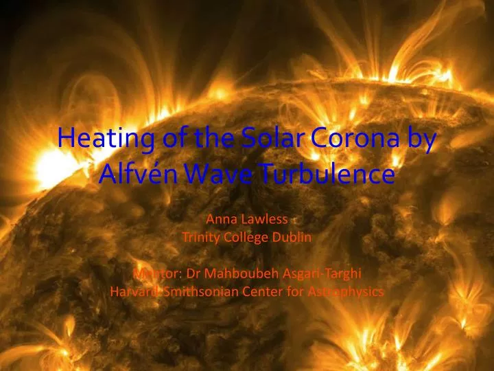
Heating of the Solar Corona by Alfvén Wave Turbulence. Anna Lawless Trinity College Dublin Mentor: Dr Mahboubeh Asgari-Targhi Harvard-Smithsonian Center for Astrophysics. The Coronal Heating Problem. Corona has a temperature significantly higher than that of the photosphere

E N D
Heating of the Solar Corona by Alfvén Wave Turbulence Anna Lawless Trinity College Dublin Mentor: DrMahboubehAsgari-Targhi Harvard-Smithsonian Center for Astrophysics
The Coronal Heating Problem • Corona has a temperature significantly higher than that of the photosphere • Seems to violate 2nd Law of Thermodynamics
Two possible solutions: Nanoflares Alfvén Wave Turbulence • Random footpoint motions cause Alfvén waves to propagate along coronal loops • Waves meet at centre of loop • Interact nonlinearly, releasing energy • Random motion of coronal loop footpoints causes braiding • Stress builds up • Magnetic field lines break up and reconnect, releasing energy Image courtesy of TRACE/NASA (Nov 1999)
Aims of This Project • To conduct comprehensive studies of generation and dissipation of Alfvén waves in the solar atmosphere in observed open and closed field lines using analytical and numerical tools. • To interpret observations and compare them to the modeling results.
Image: http://orbiterchspacenews.blogspot.com/2012/07/sounding-rocket-mission-to-observe.html Image:http://cse.ssl.berkeley.edu/stereo_solarwind/mission.html Data Sources • STEREO – employs two nearly identical space based observatories, one ahead of the earth and one behind • MDI – an instrument on the SOHO spacecraft, measures height of the transition region and magnetic field strength • EIS – a spectrometer on Hinode, provides monochromatic images of the TR and corona
Part One: Modeling • Coronal Modeling System (CMS2) program used to select and model a closed loop
evolve.f90 program used to solve differential equations Magnetic Induction Equation Plasma Equation of Motion
Braid program used to analyse the results • Computes temperature, pressure, magnetic field strength, average heating rate and other parameters along the loop
Results Model f41r1
Results Model f41r1
Open Field Line • Same analysis repeated for open field lines
Results Model f47r1
Part Two: Observations • EUV Imaging Spectrometer (EIS) – combination of multilayer telescope and spectrometer in 170-210 Å and 250-290 Å • Spectral observations used to infer plasma motions Image: http://orbiterchspacenews.blogspot.com/2012/07/sounding-rocket-mission-to-observe.html
EIS Data Fe XII – 192.394 Å 1.0 x 10⁶ K Fe XIII – 202.044 Å 1.6 x 10⁶ K Fe XV – 284.160 Å 2.0 x 10⁶ K Fe XVI – 262.980 Å 2.5 x 10⁶ K
Doppler Shifts • Source moving with speed vD relative to the observer • Emitted frequency f, emitted wavelength λ • Observed wavelength = λ ± vD/f • Change in wavelength ∆λD = vD/f = λvD/c
Doppler Width • Sources of line broadening: instrumental, thermal, non-thermal (‘microturbulent’) • Total Doppler broadening: • FWHM then given by:
Results – Closed Field Line Model f49r1 – Fe XII 192.39
Results – Closed Field Line LOS VLOS2 = Vperp2cos2θ + Vpar2 sin2θ Model f49r1 – Fe XII 192.39
Results – Open Field Line Model f47r1 – Fe XII 192.39
Results – Open Field Line Model f47r1 – Fe XII 192.39
Summary and Conclusions • In this project I modeled Alfvénwaves in both closed and open field lines • I compared the results with data from EIS • Good agreement for closed field lines • Next: focus on improving modeling techniques for open field lines and better comparisons with EIS observations
Acknowledgements • NSF grant for the Solar Physics REU Program at the SAO (AGS-1263241) • Dr. MahboubehAsgari-Targhi • Drs. Kathy Reeves and Trae Winter • The CfA and SSXG • The 2013 Solar and Astronomy REU interns Thank you!