Download

1 / 17
210 likes | 486 Vues
Human Influence on Ecosystems. Rachel Carson. Effects of Pesticides on Ecosystems. Birth of the Environmental Movement. Silent Spring. Biomagnification. As you move up through the food chain the concentration of the pollutant increases. DDT the classical Example.

E N D
Rachel Carson Effects of Pesticides on Ecosystems Birth of the Environmental Movement Silent Spring
Biomagnification As you move up through the food chain the concentration of the pollutant increases DDT the classical Example PCB’s another example
Effect of Nutrients on a Lake Ecosystem Limiting Nutrient Usually Nitrogen or Phosphorus in Aquatic ecosystems homeostasis
Note algae must live near surface so they can get light, but the decomposers live at the bottom. Mixing between layers is necessary Aerobic decomposers need oxygen supplied by algae. Algae need nutrients supplied by decomposers
Lake Stratification External Nutrient Input Algae Blooms Eutrophication
Rate of Oxygen accumulated Rate of Oxygen In Rate of Oxygen Out Rate of Oxygen Generated = - + Effect of Organic Wastes on Streams A stream may be thought of as a plug flow reactor Mass balance on dissolved oxygen
Rate of Oxygen accumulated Rate of Oxygen In (reaeration) Rate of Oxygen Consumed (deaeration) = - 0 + Oxygen is introduced into the stream by reaeration or reoxygenation There is no oxygen leaving the stream since we will assume it is unsaturated Dissolved oxygen may be produced in water by algae during Photosynthesis, but is a swift stream the algae don’t have time to grow and there is no oxygen produced in this way. Oxygen may be used by microorganisms respiration. This is called deaeration or deoxygenation. So the new mass balance is: Rate of deaeration = -k1C (first order) k1 = deaeration constant, function of type of waste, temperature, etc. Units, day-1
Rate of reaeration = k2 D (first order) k2 = reaeration constant based on characteristics of the stream and the weather Measured in field or estimated using equations such as equation on page 187 of text D = oxygen deficit = S - C S = oxygen saturation concentration, a function of temperature of the water, atmospheric oxygen concentration, and water chemistry
Maximum oxygen concentration increase with decreasing temperature
Rate of Oxygen accumulated Rate of Oxygen In (reaeration) Rate of Oxygen Consumed (deaeration) = - 0 + dD/dt = k1z - k2D z = the amount of O2 still needed by the microorganisms = L e-k1t L = ultimate oxygen demand Substitute and integrate: D = [(k1 L0)/(k2 – k1)] (e-k1t – e-k2t) = D0e-k2t D0 = the oxygen deficit at the point in the stream we call 0 L0 = the oxygen demand at the point in the stream we call 0
To find the point on the stream where the deficit, D, is the greatest we will set dD/dt = 0 and solve the equation for t: tC = [1/(k2 – k1)] ln[(k2/k1)(1 – (D0 x (k2- k1))/(k1L))] tC then is the time downstream where the oxygen concentration is at its lowest
Qp = 0.5 m3/s Tp = 26oC BODup = 48 mg/L DOp = 1.5 mg/L Qs =2.2 m3/s Ts = 12oC BODus = 13.6 mg/l V = 0.85 m/s Ds = ? Q0 = ? T0 = ? BODu0= ? D0 = ? Example A stream flows at 2.2 m3/sec with a velocity of 0.85 m/s and temperature of 12oC. The stream is saturated with dissolved oxygen, has an ultimate oxygen demand of 13.6 mg/L, and has a reaeration constant of 0.4 day-1. Treated waste from a municipal waste treatment plant is discharged to the stream. The waste stream has an ultimate BOD of 48 mg/L, a flow rate of 0.5 m3/s, a dissolved oxygen concentration of 1.5 mg/L, and a temperature of 26oC. After the waste is mixed with the stream the deaeration constant is 0.2 day –1. What is the dissolved oxygen concentration 48.3 km downstream? What is the minimum dissolved oxygen concentration, and where does it occur?
Qp = 0.5 m3/s Tp = 26oC BODup = 48 mg/L DOp = 1.5 mg/L Qs =2.2 m3/s Ts = 12 oC BODus = 13.6 mg/l V = 0.85 m/s Ds = ? Q0 = ? T0 = ? BODu0= ? D0 = ? T0 = [(QsTs) + (QpTp)]/(Qs + Qp) = [(2.2)(12) + (0.5)(26)]/(2.2 + 0.5) = 14.6oC Since the stream is saturated with DO, Ds = 0 and S = Cs =10.8oC C0 = [(QsCs) + (QpCp)]/(Qs + Qp) = [(2.2)(10.8) + (0.5)(1.5)]/(2.2 + 0.5) D0 = S0 - C0 = 9.1 mg/L Since T0 = 14.6, S0 = 10.2 mg/L D0 = 10.2 - 9.1 = 1.1 mg/L
L0 = [(Ls)(Qs) + (Lp)(Qp)]/(Qs + Qp) = [(13.6)(2.2) + (48)(0.5)]/(2.2 + 0.5) = 20 mg/L Deficit at 48.3 km: 48.3 x 10³ m/0.85 m/s = 56.8 x 10³ sec = 0.66 days D = (k1L0)/(k2 –k1) [(e-k1 t - e-k2 t)] + D0 e-k2 t = (0.2)(20)/(0.4 – 0.2)[e-0.2(0.66) – e-0.4(0.66)) + 1.1 (e-0.4 (0.66)) = 3.0 m/L C = S – D = 10.2 – 3.0 = 7.2 mg/L
tC = [1/(k2 – k1)] ln[(k2/k1)(1 – (D0 x (k2- k1))/(k1L))] = [1/(0.4 – 0.2)] ln[(0.4/0.2)(1 – (1.1(0.4-0.2)/(0.2)(20)] = 3.18 days At 3.18 Days D = (k1L0)/(k2 –k1) [(e-k1 t - e-k2 t)] + D0 e-k2 t = (0.2)(20)/(0.4 –0.2) [(e-0.2(3.18) – e-0.4(3.18))] + 1.1 e-0.4(3.18) = 5.29 mg/L C = S – D = 10.2 – 5.29 = 4.91 mg/L