Download
1 / 56
560 likes | 673 Vues
Recent progress in CO 2 flux data assimilation. Ken Davis Penn State/LSCE with D. Ricciuto, T. Hilton, A. Desai, P. Ciais, M. Reichstein, S. Piao. Outline. Introduction and history. Barriers to progress. Evaluation or assimilation?

E N D
Recent progress in CO2 flux data assimilation Ken Davis Penn State/LSCE with D. Ricciuto, T. Hilton, A. Desai, P. Ciais, M. Reichstein, S. Piao LSCE
Outline • Introduction and history. • Barriers to progress. • Evaluation or assimilation? • An example of flux data assimilation with the aim of improving predictive capacity. • Progress towards understanding the spatial and temporal statistics of ecosystem fluxes. LSCE
Introduction and history: Flux tower measurements in the story of the global carbon cycle. LSCE
Overall goals: terrestrial carbon cycle science “Top-down” methods • Quantify the non fossil fuel global carbon budget • Observe spatial and temporal patterns in the atmospheric CO2 budget and infer fluxes Diagnosis, inference “Bottom-up” methods • Build mechanistic, or “bottom-up” models that can • Reproduce observed spatial and temporal gradients in terrestrial fluxes (flux towers, atmospheric budgets). • Predict future terrestrial fluxes Attribution, prediction LSCE
Inherent spatial and temporal scales of methods of studying the carbon cycle LSCE
1950s-1980s 1990 Early 1990s Mid to late 1990s Early 2000s Atmospheric CO2 monitoring initiated. N. Hemisphere terrestrial sink of CO2 inferred. Strong interannual variability in global-scale terrestrial fluxes of CO2 observed. 20 year trends in the amplitude of the seasonal cycle of CO2 exchange observed in the N. hemisphere. Attempts at continental to regional atmospheric inversions. Forest inventories, satellite land-surface observations commence. Continuous flux tower measurements initiated at Harvard Forest. Network of flux tower sites expands rapidly. Methodological research. Many publications showing one year of flux observations from one site. Missing sink observed? Publications covering a few years of data from individual sites. Climate-driven variability in terrestrial fluxes observed? Forest inventory used to estimate large-scale, decadal C fluxes. Publications comparing single years at multiple sites. No explicit spatial component. Some publications attempt to merge multiple sites across space. time LSCE
Barriers to progress LSCE
Flux tower footprints are very small (~1km2) compared to the globe. • Neither net annual fluxes nor interannual variability in fluxes observed at flux towers can be readily linked to the observed global carbon balance. • Mechanisms remain uncertain. Attribution has not been successful at regional to global scales. ?? x 107 = 1 PgC yr-1 ?? = ± 1PgC yr-1 ?? ~1 km2 LSCE
Flux towers are limited in their time of record. Climate-driven trends and long-time scale processes are not well-constrained by these observations. • Detection of trends in flux tower time series is not clear. • Ability to predict future fluxes is suspect. Decadal or longer prediction remains highly uncertain for any spatial scale. Flux tower time series flux Multi-decade terrestrial carbon cycle model prediction and uncertainty time 5-10 years of observations LSCE
We cannot perform atmospheric inversions at small spatial and temporal scales • Too many unknowns, not enough data • We are uncertain about how to interpolate flux tower data across space • Mechanisms governing spatial variability in fluxes are uncertain Regional diagnosis of terrestrial fluxes at any time scale remains uncertain. Each grid box has a different flux for each time step. Is every flux independent in space and time? 100-1000 km domain LSCE
Potential avenues for progress Potential solution • Map fluxes over space using a numerical model aided by remote sensing and other spatial databases. Compare to atmospheric budgets. • Maintain observations, add complementary observations (e.g. forest inventory), evaluate model skill. • Study the spatial and temporal correlations in flux observations, flux-model differences. Barrier • Lack of attribution of causes of large-scale fluxes. Limited spatial scale of a flux tower footprint. • Inability to detect influence of climatic change, predict future fluxes. • Uncertainty in how to aggregate fluxes over space. Inability to diagnose regional fluxes with confidence. LSCE
Outline • Introduction and history. • Barriers to progress. • Evaluation or assimilation? • An example of flux data assimilation with the aim of improving predictive capacity. • Progress towards understanding the spatial and temporal statistics of ecosystem fluxes. LSCE
Evaluation or assimilation? Flux tower observations Terrestrial carbon cycle model Atmospheric inversion fluxes vs. vs. vs. Terrestrial model optimized to match the flux tower observations. Flux estimates optimized to all available data sources Carbon cycle data assimilation LSCE
An example of flux data assimilation with the aim of improving predictive capacity LSCE
Multi-year data assimilation at multiple flux tower sites Does data assimilation improve a terrestrial carbon cycle model’s ability to simulate diurnal, synoptic, seasonal, interannual variability in fluxes? What are the implications for predicting future fluxes? Can we simulate cross-site variability in fluxes? Can we use a common set of model parameters for multiple sites? Are any model parameters poorly-constrained by the flux data? What happens to carbon pools after assimilation? Ricciuto, Ph.D. dissertation, 2006. LSCE
Assimilation technique • This is a potentially nonconvex problem, thus we chose a global optimization algorithm, Stochastic Evolutionary Ranking Strategy (SRES) • Stochastic – difficult to guarantee convergence • Relatively fast method to find very good solution • No parametric uncertainty (unlike MCMC) • Method: • - Twiddle all the knobs in the model until it matches all of the data. • Start with initial population (parameter sets) • Evaluate goodness of fit (likelihood function) • Select best-fitting members (parameter sets) • Mutate these members, repeat until convergence “apparent” • Run three times for each tower, compare solutions LSCE
Tower sites Site-years analyzed (37 total) WLEF: 1997-2004 Harvard: 1992-2003 Howland: 1996-2003 UMBS: 1999-2003 M. Monroe: 1999-2003 LSCE
GPP (NL,BL) Forcing: wind, [CO2], PAR, Tair, precip NPP (NL,BL) Ra Ra Leaf (NL) Leaf (BL) NEE Wood (BL) Wood (NL) RH Root (NL) Root (BL) Soil carbon (CS) Simplified TRIFFID Model LSCE
Why TRIFFID? • Dynamic Global Vegetation Model: Contains longer-term processes essential for decadal scale predictions. • Used in Cox et al. (2000) – strong feedbacks. Are model parameters realistic? Is model structure appropriate? Cox et al. (2000) Cox et al. (2000) LSCE Friedlingstein et al. (2006) Friedlingstein et al. (2006)
Twenty-two of TRIFFID’s (40?) parameters were chosen (by the seats of our pants) for optimization. Optimization with all parameters (one test case) did not significantly change our results. LSCE
Multi-year data assimilation at multiple flux tower sites Does data assimilation improve a terrestrial carbon cycle model’s ability to simulate diurnal, synoptic, seasonal, interannual variability in fluxes? Yes! No! What are the implications for predicting future fluxes? Little confidence in long-term predictions if interannual variability cannot be simulated after assimilating all available data. LSCE
Model performance:Synoptic variability Our model reproduces daily sums of NEE reasonably well (example month: Sep 1997) LSCE
Timescales of modeled and observed fluxes • Analysis using SIPNET model: MCMC optimization with 26 parameters • Fluxes at Harvard Forest: • Largest variance in diurnal and seasonal cycles • Optimized model fits these well • Interannual variability: • worst timescale for performance • Model underestimates • consistent with TRIFFID results Diurnal Seasonal Synoptic Interannual LSCE Braswell et al. (2005)
Hypotheses: The model has a structural flaw that prevents it from being able to reproduces observed interannual variability in fluxes. Our best guess. (If so, maybe the process that is missing is something that is very local, and the model does fine at large spatial scales? Probably not the case.) OR The observed interannual flux variability is insignificant or erroneous. Probably not the case. LSCE
Significant Interannual variability at WLEF • fff Uncertainty = gap-filling uncertainty + turbulent sampling uncertainty.Random error: about 20 gC m-2 The range of interannual variability is therefore statistically significant at the 95% level. Quantified systematic errors: Loss of very low frequency fluxes, choice of low-turbulence screening threshold, changes in flux levels: Also about 20 gC m-2 (for IAV). LSCE
Eddy-covariance is a good method for characterizing interannual variability in fluxes. • Sums may be biased due to advection, other systematic errors, but these (unquantified systematic) errors will not change much from year to year. LSCE
Observed interannual variability: only local processes? Probably not. Gap-filled fluxes from the 5 sites used in TRIFFID analysis Harvard and Howland: Coherent between 1996 and 2000, then breaks down. UMBS and Morgan Monroe: coherent (similar PFT, climate) WLEF: 2002 missing, coherent with UMBS and Morgan Monroe LSCE
Multi-year data assimilation at multiple flux tower sites Can we simulate cross-site variability in fluxes? Can we use a common set of model parameters for multiple sites? Yes to both questions, if we let soil carbon and leaf nitrogen (maximum photosynthetic rate) vary across sites. this implies that these are quantities that must be mapped accurately in space and used as model inputs. if they varied from year-to-year, we could also fit interannual variability, but what is the mechanism? Ricciuto, Ph.D. dissertation, 2006. LSCE
Model performance: Cross-site variability • Site-specific variables, held constant in time. • Soil carbon • Leaf nitrogen (Vmax) • Forest structure (needleaf or broadleaf, canopy height) LSCE
Multi-year data assimilation at multiple flux tower sites Are any model parameters poorly-constrained by the flux data? Yes. Respiration parameters. What happens to carbon pools after assimilation? Out of equilibrium. Is this realistic? We don’t know… Ricciuto, Ph.D. dissertation, 2006. LSCE
Convergence diagnostics • Objective function = -1*log(likelihood) • 3 runs generally converge for each site, but some slight disagreement • Some model parameters converge • photosynthesis • phenology • Some are poorly constrained • Heterotrophic respiration • Autotrophic respiration LSCE
Twenty-two of TRIFFID’s (40?) parameters were chosen (by the seats of our pants) for optimization. Optimization with all parameters (one test case) did not significantly change our results. LSCE
How do we diagnose the potential model structural error? • One way - limit the number of processes the model simulates - for example, cut out the soil hydrology by imposing observed soil moisture. LSCE
1950s-1980s 1990 Early 1990s Mid to late 1990s Early 2000s Atmospheric CO2 monitoring initiated. N. Hemisphere terrestrial sink of CO2 inferred. Strong interannual variability in global-scale terrestrial fluxes of CO2 observed. 20 year trends in the amplitude of the seasonal cycle of CO2 exchange observed in the N. hemisphere. Attempts at continental to regional atmospheric inversions. Forest inventories, satellite land-surface observations commence. Continuous flux tower measurements initiated at Harvard Forest. Network of flux tower sites expands rapidly. Methodological research. Many publications showing one year of flux observations from one site. Missing sink observed? Publications covering a few years of data from individual sites. Climate-driven variability in terrestrial fluxes observed? Forest inventory used to estimate large-scale, decadal C fluxes. Publications comparing single years at multiple sites. No explicit spatial component. Some publications attempt to merge multiple sites across space. time LSCE
Potential avenues for progress Potential solution • Map fluxes over space using a numerical model aided by remote sensing and other spatial databases. Compare to atmospheric budgets. • Maintain observations, add complementary observations (e.g. forest inventory), evaluate model skill. • Study the spatial and temporal correlations in flux observations, flux-model differences. Barrier • Lack of attribution of causes of large-scale fluxes. Limited spatial scale of a flux tower footprint. • Inability to detect influence of climatic change, predict future fluxes. • Uncertainty in how to aggregate fluxes over space. Inability to diagnose regional fluxes with confidence. LSCE
Outline • Introduction and history. • Barriers to progress. • Evaluation or assimilation? • An example of flux data assimilation with the aim of improving predictive capacity. • Progress towards understanding the spatial and temporal statistics of ecosystem fluxes. LSCE
Sabbatical plans • Examine the space-time statistics of flux observations and flux-model residuals for selected study areas: • ChEAS - many towers, very different stand types, very similar climate - nearly colocated • Plant functional type clusters - same stand types, varying climate/spatial separation. Europe, North America. • Use both optimized and non-optimized ecosystem models. LSCE
Sabbatical results • Incomplete driver data preparation (but I haven’t given up!) • A nice workshop - plans to initiate FLUXCOM • A couple of good plots from my students • A bit of ORCHIDEE-AmeriFlux comparison • Lots of good CO2-relevant discussions of boundary layer meteorology (which I hope to continue) • Many family dinners together • My kids learned a lot of French! LSCE
Observed interannual variability: only local processes? Probably not. Gap-filled fluxes from the 5 sites used in TRIFFID analysis Harvard and Howland: Coherent between 1996 and 2000, then breaks down. UMBS and Morgan Monroe: coherent (similar PFT, climate) WLEF: 2002 missing, coherent with UMBS and Morgan Monroe LSCE
Northern Wisconsin - ChEAS (Chequamegon Ecosystem-Atmosphere Study) 18 flux measurement sites and the WLEF trace gas measurements First “ring of towers” regional inversion experiment Abundant ancillary data - remote sensing of surface, ground-based plant physiological and biometric data, atmospheric profiling LSCE
7 day block averaged fluxes 1 year block averaged fluxes LSCE
Another view of spatial correlation of fluxes Chevallier et al (2006): no correlation at any spatial scale in model-data residuals Daily average fluxes Mixed vegetation types Model is not optimized for the observed fluxes LSCE
Continental Interannual Index Water Availability Ea/Ep (mm/mm) Mean annual temperature (°C) Climatic Gradients in European Fluxes Reichstein, Papale et al. GRL, in press cf. also Valentini et al. (2000) Law et al. (2002) Southern sites - water limited Northern sites - temperature limited LSCE
Climatic Gradients in North American Fluxes Color indicates plant functional type. Each small symbol is a site-year. LSCE
Findings - flux data only Very similar flux vs. climate spatial slopes over Europe and North America. Both GPP and TER positively correlate with annual temperature and water availability. Cross-site NEE dependency on climate is weak (compensating gradients of TER, GPP - effects of management, for example, become more prominent). Results broadly similar to Law et al (2002), but this analysis limited to forested systems, benefits from longer time series. Interannual variability at sites does not appear to follow the cross-site climatic gradient in fluxes. Does ORCHIDEE produce similar spatial gradients? Analyses underway. LSCE
What controls IAV in GPP ? Model suggests that GPP variability is determined by : Temperature in the North and by rainfall in the South Maps of R2(GPP-Temperature) minus R2(GPP-Precipitation) Is this also observed in eddy-covariance time series ? Analyses in progress. LSCE