Download
1 / 48
850 likes | 2.33k Vues
Production Planning and Control Inventory Management. Dr. Lotfi K. Gaafar. Production Planning and Control. The Production Control System. Sales and order entry. Demand forecasting. Customer. Shop-floor scheduling and control. Materials requirement planning. Aggregate planning.

E N D
Production Planning and Control Inventory Management Dr. Lotfi K. Gaafar Production Planning and Control- Inventory Management(1)
Production Planning and Control The Production Control System Sales and order entry Demand forecasting Customer Shop-floor scheduling and control Materials requirement planning Aggregate planning Shipping and receiving Production Inventory management Inventory Vendors Production Planning and Control- Inventory Management(2)
Demand Management • Basic Problem: establish an interface between the customer and the plant floor, that supports both competitive customer service and workable production schedules. • Issues: • Customer Lead Times: shorter is more competitive. • Customer Service: on-time delivery. • Batching: grouping like product families can reduce lost capacity due to setups. • Interface with Scheduling: customer due dates are are an enormously important control in the overall scheduling process. Production Planning and Control- Inventory Management(3)
Why Manage Inventory? • Total $ investment on in inventories is $1.37 trillion (last quarter of 1999) • 34% in Manufacturing • 26% in Retail • 22% in Wholesale • 8% in Farm • 10% in Other 82% of the total Production Planning and Control- Inventory Management(4)
Why Manage Inventory? • In 1998, American companies spent $898 billion in logistics-related activities (or 10.6% of Gross Domestic Product). • Transportation 58% • Inventory 38% • Management 4% • By effectively managing inventory: • Xerox eliminated $700 million inventory from its supply chain • Wal-Mart became the largest retail company utilizing efficient inventory management • GM has reduced parts inventory and transportation costs by 26% annually Production Planning and Control- Inventory Management(5)
Customers, demand centers sinks Field Warehouses: stocking points Sources: plants vendors ports Regional Warehouses: stocking points Supply Inventory & warehousing costs Production/ purchase costs Transportation costs Transportation costs Inventory & warehousing costs Production Planning and Control- Inventory Management(6)
Why Manage Inventory? • By not managing inventory successfully • In 1994, “IBM continues to struggle with shortages in their ThinkPad line” (WSJ, Oct 7, 1994) • In 1993, “Liz Claiborne said its unexpected earning decline is the consequence of higher than anticipated excess inventory” (WSJ, July 15, 1993) • In 1993, “Dell Computers predicts a loss; Stock plunges. Dell acknowledged that the company was sharply off in its forecast of demand, resulting in inventory write downs” (WSJ, August 1993) Production Planning and Control- Inventory Management(7)
Inventory • Where do we hold inventory? • suppliers and manufacturers • warehouses and distribution centers • retailers • Types of Inventory • WIP and subassemblies • raw materials • finished goods • Why do we hold inventory? (Short answer) • Economies of scale • Uncertainty in supply and demand Production Planning and Control- Inventory Management(8)
Why do we hold inventory? • Economies of scale • Uncertainty in supply and demand • Speculation • Transportation • Smoothing production/purchasing • Logistics • Cost of controlling inventory Production Planning and Control- Inventory Management(9)
Decisions to Make • We have to decide • How often we review the inventory • When we should issue a (replenishment/production) order • How large the order should be Production Planning and Control- Inventory Management(10)
Characteristics of Inv. Systems • Demand • Constant (level) or variable • Deterministic (known) or Stochastic (random or uncertain) • Lead Time • Review Time • Continuous or periodic review • Excess Demand • Backordered or lost • Changing inventory Production Planning and Control- Inventory Management(11)
Relevant Costs • Unit value or unit variable cost (c) • Cost of making a part available for usage • Purchase + Freight + Mfg. Costs • Usually different from “accounting” cost • Should include more than just book value Production Planning and Control- Inventory Management(12)
Relevant Costs • Holding cost (cost of carrying in inv.) • Opportunity costs of the money tied to inventory (I = ic), where i is the available rate of return on investment (may use IRR). • Warehousing and Handling (cost of providing space to store items, counting and moving items in the warehouse) • Deterioration, damage, obsolescence • Insurance and taxes • W: Warehousing cost, $ per item per year Production Planning and Control- Inventory Management(13)
Relevant Costs Inv. Avg. inv. level Time, t 1 2 Production Planning and Control- Inventory Management(14)
Relevant Costs • Ordering or Setup Cost (P) • Fixed cost • Independent of the size of the replenishment or production order • Ordering forms, phone calls, other communication costs, receiving, inspection, cost of interrupted production, opportunity cost of lost time, etc. Production Planning and Control- Inventory Management(15)
EOQ History • Introduced in 1913 by Ford W. Harris, “How Many Parts to Make at Once” • Interest on capital tied up in wages, material and overhead sets a maximum limit to the quantity of parts which can be profitably manufactured at one time; “set-up” costs on the job fix the minimum. Experience has shown one manager a way to determine the economical size of lots. • Early application of mathematical modeling to Scientific Management Production Planning and Control- Inventory Management(16)
EOQ Modeling Assumptions • 1.Production is instantaneous – there is no capacity constraint and the entire lot is produced simultaneously. • 2.Delivery is immediate – there is no time lag between production and availability to satisfy demand. • 3.Demand is deterministic – there is no uncertainty about the quantity or timing of demand. • 4.Demand is constant over time – in fact, it can be represented as a straight line, so that if annual demand is 365 units this translates into a daily demand of one unit. • 5.A production run incurs a fixed setup cost – regardless of the size of the lot or the status of the factory, the setup cost is constant. • 6.Products can be analyzed singly – either there is only a single product or conditions exist that ensure separability of products. Production Planning and Control- Inventory Management(17)
EOQ Model • Time unit: one year • Total Cost = setup cost + opportunity cost + Warehousing cost, total cost is calculated per unit. • Purchase Cost Constant • Opportunity cost is always based on average quantity • Warehousing cost may be based on average quantity for mixed storage areas, or on maximum quantity for dedicated storage. • Goal: Find the order quantity that minimizes total costs • General Equation for dedicated storage for mixed storage Production Planning and Control- Inventory Management(18)
EOQ Model Assumptions: • No Stockouts • Order when no inventory • Order size determines policy Inventory Qavg = Q/2 Order Quantity Q Avg. Inventory (Qavg) Production Planning and Control- Inventory Management(19)
EOQ Model Total Cost Holding Cost Order Cost Optimal Order Quantity, Q* Production Planning and Control- Inventory Management(20)
EOQ Model for dedicated storage for mixed storage By differentiation: for dedicated storage for mixed storage Production Planning and Control- Inventory Management(21)
EOQ Model Example: Zartex Co. produces fertilizer to sell to wholesalers. One raw material – calcium nitrate – is purchased from a nearby supplier at $22.50 per ton. Zartex estimates it will need 5,750,000 tons of calcium nitrate next year. The annual carrying cost for this material is 40% of the acquisition cost, and the ordering cost is $595. a) What is the most economical order quantity? b) How many orders will be placed per year? c) How much time will elapse between orders? Production Planning and Control- Inventory Management(22)
EOQ Model • Tradeoff between set-up costs and holding costs when determining order quantity. In fact, we order so that these costs are equal per unit time • Total Cost is not particularly sensitive to the optimal order quantity Production Planning and Control- Inventory Management(23)
EOQ Observations • Batching causes inventory (i.e., larger lot sizes translate into more stock). • Under specific modeling assumptions the lot size that optimally balances holding and setup costs is given by the square root formula: • Total cost is relatively insensitive to lot size (so rounding for other reasons, like coordinating shipping, may be attractive). • carrying cost (cc) = I + W or cc = I + 2W Production Planning and Control- Inventory Management(24)
EOQ Trade-off • Two interpretations: • If you order more (larger Q), you incur higher inventory cost, but less setup cost • If you order less frequently, you incur larger inventory cost, but less setup cost • The trade-off is not linear! Production Planning and Control- Inventory Management(25)
Economic Manufacturing Quantity (EMQ) • What happens when there is finite production rate? • A: production rate (in units per year) • A>D (demand rate per year). Why? • What happens if you keep producing? • The inventory will keep growing forever with a rate of A-D. • There are many possible scenarios. The common two are: • A: Start producing Q when inventory reaches zero. • B: Start producing a batch of Q so that the quantity is finished when the previous batch is consumed. Production Planning and Control- Inventory Management(26)
EMQ- Scenario A Start producing Q when inventory reaches zero at the rate of A parts per time unit. Consumption is continuous at the rate of D parts per time unit until inventory reaches zero, at which time production starts again. Inv Q QM TA Time TC Start Prod. Start Prod. Stop Prod. Production Planning and Control- Inventory Management(27)
EMQ- Scenario A for dedicated storage for mixed storage By differentiation: for dedicated storage for mixed storage Production Planning and Control- Inventory Management(28)
EMQ- Scenario B Start producing a batch of Q, at the rate of A parts per time unit, so that the quantity is finished when the previous batch is consumed. Consumption is continuous at the rate of D parts per time unit. Inventory never reaches zero. QMis the minimum inventory level. Inv Q QM QM TA Start Prod. Start Prod. T Stop Prod. Time Production Planning and Control- Inventory Management(29)
EMQ- Scenario B for dedicated storage for mixed storage By differentiation: for dedicated storage for mixed storage Production Planning and Control- Inventory Management(30)
Resource Constrained Multiple Product Systems • Another EOQ assumption: • Even if you have multiple items to worry, you can analyze them separately • What happens if the items share capacitated resources? • Budget • Machines • Personnel • Space, etc. Production Planning and Control- Inventory Management(31)
MedEquip Example Costs • D = 1000 racks per year • c = $250 • P = $500 (estimated from supplier’s pricing) • cc = (0.1)($250) + 10 = $35 per unit per year Production Planning and Control- Inventory Management(32)
Costs in EOQ Model Production Planning and Control- Inventory Management(33)
Dynamic Lot Sizing • Another EOQ assumption: • Demand is constant over time • Dynamic Lot Sizing relaxes this assumption • Demand is changing over time • But demand in each period is known (so still deterministic). Production Planning and Control- Inventory Management(34)
Dynamic Lot Sizing • Examples: • MRP • Firm orders and contracts for future periods • Seasonal demand patterns • Demand with trend (increasing or decreasing over time) Production Planning and Control- Inventory Management(35)
Dynamic Lot Sizing • Example: • Other data • Beginning inventory: 0 • Setup cost: $150 • Inventory carrying cost: $2 per unit per period Production Planning and Control- Inventory Management(36)
Dynamic Lot Sizing • Issues: • Determine a planning horizon • Calculate total cost over the planning horizon • Implementing decisions over time • Rolling horizon concept • Discrete demand vs. Continuous demand • Discrete Replenishments vs. Any-time replenishments Production Planning and Control- Inventory Management(37)
Dynamic Lot Sizing • Quick Solutions • Order every period exactly as much as you need • Lot-for-Lot • Determine a fixed order quantity and order when you need to order (i.e., when on-hand inventory is less than the next period’s demand) • Example: EOQ • Order constant time-supply (i.e., order the amount sufficient to cover total demand in next three months) Production Planning and Control- Inventory Management(38)
Dynamic Lot Sizing • Lot-for-lot solution: Total Cost = 150 + 10 * 150 = $1650 Production Planning and Control- Inventory Management(39)
Dynamic Lot Sizing • Other heuristics: • EOQ as a Time Supply • Periodic Order Quantity (POQ) • Part-Period Balancing (PPB) • Silver-Meal (or Least Period Cost) Production Planning and Control- Inventory Management(40)
Dynamic Lot Sizing • Example • Calculate EOQ: • Average demand per week = ____ • Holding cost per unit per week = ____ • EOQ = ____ • Total Holding and Setup Cost = ____ Production Planning and Control- Inventory Management(41)
Dynamic Lot Sizing- EOQ Total Cost = 642 + 4 * 150 = $1242 Production Planning and Control- Inventory Management(42)
Dynamic Lot Sizing - POQ • Periodic Order Quantity • Calculate EOQ using Average Demand • Calculate Time Supply and round it to the nearest integer • In each replenishment, order to cover that many periods’ demand • Fixed order interval, but different quantity in each replenishment Production Planning and Control- Inventory Management(43)
Dynamic Lot Sizing - POQ Total Cost = 422 + 4 * 150 = $1022 Production Planning and Control- Inventory Management(44)
Dynamic Lot Sizing - PPB • Part-Period Balancing • Select the number of periods covered by the replenishment such that the total inventory carrying costs are as close as possible to the setup cost. Production Planning and Control- Inventory Management(45)
Dynamic Lot Sizing - PPB Total Cost = 422 + 4 * 150 = $1022 Production Planning and Control- Inventory Management(46)
Dynamic Lot Sizing - SM • Silver-Meal (SM) Heuristic • Minimize total relevant costs per unit time for the duration of the replenishment quantity. • Replenishment quantity Q should last for an integer number of periods: cover the total demand in periods 1 through T (decision variable T) • Min (Setup Cost + Inv Cost through T) / T • Q = D1 + … + DT • Total Relevant Cost through T: TRC(T) • Select T such that TRC(T)/T is minimized. Production Planning and Control- Inventory Management(47)
Dynamic Lot Sizing - SM Total Cost = 366 + 4 * 150 = $966 Production Planning and Control- Inventory Management(48)