Download
1 / 125
1.25k likes | 1.26k Vues
Supplemental Lecture Notes. 1 - Introduction 2 - Exploratory Data Analysis 3 - Probability Theory 4 - Classical Probability Distributions 5 - Sampling Distrbns / Central Limit Theorem 6 - Statistical Inference 7 - Correlation and Regression (8 - Survival Analysis).

E N D
Supplemental Lecture Notes 1 - Introduction 2 - Exploratory Data Analysis 3 - Probability Theory 4 - Classical Probability Distributions 5 - Sampling Distrbns / Central Limit Theorem 6 - Statistical Inference 7 - Correlation and Regression (8 - Survival Analysis)
What is the connection between probability and random variables? Events (and their corresponding probabilities) that involve experimental measurements can be described by random variables.
POPULATION Discrete random variable X Example: X = Cholesterol level (mg/dL) x1 x3 x2 x6 x4 …etc…. x5 xn SAMPLE of size n
POPULATION Discrete random variable X Example: X = Cholesterol level (mg/dL) X “Density” Probability Histogram Total Area = 1 p(x)= Probability that the random variable X is equal to a specific value x, i.e., p(x) = P(X = x) “probability mass function” (pmf) | x
Consider the following discrete random variable… Example: X = “value shown on a single random toss of a fair die (1, 2, 3, 4, 5, 6)” Xis said to be uniformly distributed over the values 1, 2, 3, 4, 5, 6. Probability Histogram P(X = x) Total Area = 1 Density f(x) X “What is the probability of rolling a 4?”
Consider the following discrete random variable… Example: X = “value shown on a single random toss of a fair die (1, 2, 3, 4, 5, 6)” Xis said to be uniformly distributed over the values 1, 2, 3, 4, 5, 6. Probability Histogram P(X = x) Total Area = 1 Density f(x) X “What is the probability of rolling a 4?”
POPULATION Discrete random variable X Example: X = Cholesterol level (mg/dL) X Probability Histogram Total Area = 1 F(x)= Probability that the random variable X is less than or equal to a specific value x, i.e., F(x) = P(Xx) “cumulative distribution function” (cdf) | x
Motivation ~ Consider the following discrete random variable… Example: X = “value shown on a single random toss of a fair die (1, 2, 3, 4, 5, 6)” Xis said to be uniformly distributed over the values 1, 2, 3, 4, 5, 6. Cumulative distribution P(Xx)
Motivation ~ Consider the following discrete random variable… Example: X = “value shown on a single random toss of a fair die (1, 2, 3, 4, 5, 6)” Xis said to be uniformly distributed over the values 1, 2, 3, 4, 5, 6. Cumulative distribution P(Xx) “staircase graph” from 0 to 1
POPULATION Discrete random variable X Example: X = Cholesterol level (mg/dL) X Calculating “interval probabilities”… F(b)= P(Xb) F(a–)= P(Xa–) F(b) – F(a–) = P(Xb) – P(Xa–) = P(aXb) p(x) | a– | b | a
POPULATION Discrete random variable X Example: X = Cholesterol level (mg/dL) X Calculating “interval probabilities”… F(b)= P(Xb) F(a–)= P(Xa–) F(b) – F(a–) = P(Xb) – P(Xa–) FUNDAMENTAL THEOREM OF CALCULUS (discrete form) = P(aXb) p(x) | a– | b | a
POPULATION Discrete random variable X Example: X = Cholesterol level (mg/dL) X Calculating “interval probabilities”… F(b)= P(Xb) F(a–)= P(Xa–) Hey!!! What about the population mean and the population variance 2 ??? F(b) – F(a–) = P(Xb) – P(Xa–) FUNDAMENTAL THEOREM OF CALCULUS (discrete form) = P(aXb) p(x) | a– | b | a
POPULATION Discrete random variable X Example: X = Cholesterol level (mg/dL) • Population mean Also denoted by E[X], the “expected value” of the variable X. • Population variance Just as the sample meanand sample variances2were used to characterize “measure of center” and “measure of spread” of a dataset, we can now define the “true” population meanand population variance 2, using probabilities.
POPULATION Discrete random variable X Example: X = Cholesterol level (mg/dL) • Population mean Also denoted by E[X], the “expected value” of the variable X. • Population variance Just as the sample meanand sample variances2were used to characterize “measure of center” and “measure of spread” of a dataset, we can now define the “true” population meanand population variance 2, using probabilities.
Example 1: POPULATION Discrete random variable X Example: X = Cholesterol level (mg/dL) 1/2 1/3 1/6 250 500
Example 2: POPULATION Discrete random variable X Example: X = Cholesterol level (mg/dL) Equally likelyoutcomes result in a “uniform distribution.” 1/3 1/3 1/3 (clear from symmetry) 210 600
Probability Table Probability Histogram POPULATION Total Area = 1 Discrete random variable X X Frequency Table Density Histogram x1 x3 x2 x6 x4 Total Area = 1 …etc…. x5 xn X SAMPLE of size n
Probability Table Probability Histogram POPULATION ? Total Area = 1 Discrete random variable X Continuous X Frequency Table Density Histogram x1 x3 x2 x6 x4 Total Area = 1 …etc…. x5 xn X SAMPLE of size n
Example 3: TWO INDEPENDENT POPULATIONS X1 = Cholesterol level (mg/dL) X2 = Cholesterol level (mg/dL) 2 = 210 22 = 600 1 = 250 12 = 500 NOTE: By definition, this is the sample space of the experiment! NOTE: By definition, this is the sample space of the experiment! What are the probabilities of the corresponding events “D = d” for d = -30, 0, 30, 60, 90? D = X1 – X2 ~ ???
Example 3: TWO INDEPENDENT POPULATIONS X1 = Cholesterol level (mg/dL) X2 = Cholesterol level (mg/dL) 2 = 210 22 = 600 1 = 250 12 = 500 The outcomes of Dare NOT EQUALLY LIKELY!!! D = X1 – X2 ~ ??? NO!!!
Example 3: TWO INDEPENDENT POPULATIONS X1 = Cholesterol level (mg/dL) X2 = Cholesterol level (mg/dL) 2 = 210 22 = 600 1 = 250 12 = 500 D = X1 – X2 ~ ???
Example 3: TWO INDEPENDENT POPULATIONS X1 = Cholesterol level (mg/dL) X2 = Cholesterol level (mg/dL) 2 = 210 22 = 600 1 = 250 12 = 500 D = X1 – X2 ~ ???
Example 3: TWO INDEPENDENT POPULATIONS Probability Histogram X1 = Cholesterol level (mg/dL) X2 = Cholesterol level (mg/dL) 2 = 210 22 = 600 1 = 250 12 = 500 6/18 5/18 3/18 3/18 1/18 D = X1 – X2 ~ ??? What happens if the two populations are dependent? Later…
Example 3: TWO INDEPENDENT POPULATIONS Probability Histogram X1 = Cholesterol level (mg/dL) X2 = Cholesterol level (mg/dL) 2 = 210 22 = 600 2 = 210 22 = 600 1 = 250 12 = 500 1 = 250 12 = 500 6/18 5/18 3/18 3/18 1/18 D = (-30)(1/18) + (0)(3/18) + (30)(6/18) + (60)(5/18) + (90)(3/18) = 40 D = X1 – X2 ~ ??? D = 1 – 2 D2 = (-70)2(1/18) + (-40)2(3/18) + (-10)2(6/18) + (20)2(5/18) + (50)2(3/18) = 1100 D2 = 12 + 22
General: TWO INDEPENDENT POPULATIONS IF the two populations are dependent… Probability Histogram X1 = Cholesterol level (mg/dL) X1 X2 = Cholesterol level (mg/dL) X2 …then this formula still holds, BUT…… 2 = 210 22 = 600 2 = 210 22 = 600 1 = 250 12 = 500 1 = 250 12 = 500 6/18 5/18 3/18 3/18 1/18 Mean (X1 – X2) = Mean (X1) – Mean (X2) D = (-30)(1/18) + (0)(3/18) + (30)(6/18) + (60)(5/18) + (90)(3/18) = 40 D = X1 – X2 ~ ??? D = 1 – 2 Var (X1 – X2) = Var (X1) + Var (X2) D2 = (-70)2(1/18) + (-40)2(3/18) + (-10)2(6/18) + (20)2(5/18) + (50)2(3/18) = 1100 – 2 Cov (X1, X2) These two formulas are valid for continuous as well as discrete distributions. D2 = 12 + 22
NOTICE TO STAT 324 • Slides 29-41 contain more details on properties of Expected Values. They are not required for Stat 324, but if you are experiencing difficulty with the formulas, you may find them of some benefit. • Special note regarding Slide 41: Similar to the “alternate computational formula” for sample variance s2, such a formula also exists for population variance σ2, derived there. Stat 324 material picks up with the Binomial Distribution.
POPULATION Discrete random variable X Example: X = Cholesterol level (mg/dL) General Properties of “Expectation” of X Suppose X is transformed to another random variable, say h(X). Then by def,
POPULATION Discrete random variable X Example: X = Cholesterol level (mg/dL) General Properties of “Expectation” of X Suppose X is constant, say b, throughout entire population… b Then by def,
POPULATION Discrete random variable X Example: X = Cholesterol level (mg/dL) General Properties of “Expectation” of X Suppose X is constant, say b, throughout entire population… Then…
POPULATION Discrete random variable X Example: X = Cholesterol level (mg/dL) General Properties of “Expectation” of X Multiply X by any constant a… a Then by def,
POPULATION Discrete random variable X Example: X = Cholesterol level (mg/dL) General Properties of “Expectation” of X Multiply X by any constant a… Then… i.e.,…
POPULATION Discrete random variable X Example: X = Cholesterol level (mg/dL) General Properties of “Expectation” of X Multiply X by any constant a… Add any constant b to X… Then… i.e.,…
POPULATION Discrete random variable X Example: X = Cholesterol level (mg/dL) General Properties of “Expectation” of X Multiply X by any constant a… Add any constant b to X… Then… i.e.,…
POPULATION Discrete random variable X Example: X = Cholesterol level (mg/dL) General Properties of “Expectation” of X
POPULATION Discrete random variable X Example: X = Cholesterol level (mg/dL) General Properties of “Expectation” of X Multiply X by any constant a… then X is also multiplied by a.
POPULATION Discrete random variable X Example: X = Cholesterol level (mg/dL) General Properties of “Expectation” of X Multiply X by any constant a… then X is also multiplied by a. i.e.,… i.e.,…
POPULATION Discrete random variable X Example: X = Cholesterol level (mg/dL) General Properties of “Expectation” of X Add any constant b to X… then b is also added to X.
POPULATION Discrete random variable X Example: X = Cholesterol level (mg/dL) General Properties of “Expectation” of X Add any constant b to X… then b is also added to X. i.e.,… i.e.,…
POPULATION Discrete random variable X Example: X = Cholesterol level (mg/dL) General Properties of “Expectation” of X
POPULATION Discrete random variable X Example: X = Cholesterol level (mg/dL) General Properties of “Expectation” of X This is the analogue of the “alternate computational formula” for the sample variance s2.
~ The Binomial Distribution ~ • Used only when dealing with binary outcomes (two categories: “Success” vs. “Failure”), with a fixed probability of Success () in the population. • Calculates the probability of obtaining any given number of Successes in a random sample of n independent “Bernoulli trials.” • Has many applications and generalizations, e.g., multiple categories, variable probability of Success, etc.
For any randomly selected individual, define a binary random variable: POPULATION 40% Male, 60% Female RANDOMSAMPLE n = 100 Discrete random variable X = # Males in sample (0, 1, 2, 3, …, 99, 100) How can we calculate the probability of How can we calculate the probability of P(X = x), for x = 0, 1, 2, 3, …,100? p(x) = P(X = x), for x = 0, 1, 2, 3, …,100? P(X = 0), P(X = 1), P(X = 2), …, P(X = 99), P(X = 100)? p(x) = F(x) = P(X≤x), for x = 0, 1, 2, 3, …,100?
For any randomly selected individual, define a binary random variable: POPULATION 40% Male, 60% Female RANDOMSAMPLE n = 100 Discrete random variable X = # Males in sample (0, 1, 2, 3, …, 99, 100) Example: How can we calculate the probability of p(25) = P(X = 25)? P(X = x), for x = 0, 1, 2, 3, …,100? p(x) = Solution: F(x) = P(X≤x), for x = 0, 1, 2, 3, …,100? Solution: Model the sample as a sequence of independent coin tosses, with 1 = Heads (Male), 0 = Tails (Female), where P(H) = 0.4, P(T) = 0.6 .… etc….
How many possible outcomes of n = 100tosses exist? How many possible outcomes of n = 100tosses exist withX = 25Heads? … X = 25Heads: { H1, H2, H3,…, H25 } HOWEVER… permutations of 25 among 100 There are 100 possible open slots for H1 to occupy. For each one of them, there are 99 possible open slots left for H2 to occupy. For each one of them, there are 98 possible open slots left for H3 to occupy. …etc…etc…etc… For each one of them, there are 77 possible open slots left for H24 to occupy. For each one of them, there are 76 possible open slots left for H25 to occupy. Hence, there are ?????????????????????? possible outcomes. 100 99 98 … 77 76 This value is the number of permutations of the coins, denoted 100P25.
How many possible outcomes of n = 100tosses exist? How many possible outcomes of n = 100tosses exist withX = 25Heads? X = 25Heads: { H1, H2, H3,…, H25 } 100 99 98 … 77 76 HOWEVER… permutations of 25 among 100 This number unnecessarily includes the distinct permutations of the 25 among themselves, all of which have Heads in the samepositions. For example: We would not want to count this as a distinct outcome.
How many possible outcomes of n = 100tosses exist? How many possible outcomes of n = 100tosses exist withX = 25Heads? X = 25Heads: { H1, H2, H3,…, H25 } 100 99 98 … 77 76 HOWEVER… permutations of 25 among 100 This number unnecessarily includes the distinct permutations of the 25 among themselves, all of which have Heads in the samepositions. 25 24 23 … 3 2 1 How many is that? By the same logic…... “25 factorial” - denoted 25! 100 99 98 … 77 76 25 24 23 … 3 2 1 = 100!_ 25! 75! R: choose(100, 25) Calculator: 100 nCr 25 “100-choose-25” - denoted or 100C25 This value counts the number of combinations of 25 Heads among 100 coins.
How many possible outcomes of n = 100tosses exist? How many possible outcomes of n = 100tosses exist withX = 25Heads? Answer: What is the probability of each such outcome? Recall that, per toss, P(Heads) = = 0.4 P(Tails) = 1 – = 0.6 Answer: Via independencein binary outcomes between any two coins, 0.4 0.6 0.6 0.4 0.6 … 0.6 0.4 0.4 0.6 = . Therefore, the probability P(X = 25) is equal to……. R: dbinom(25, 100, .4)
How many possible outcomes of n = 100tosses exist? How many possible outcomes of n = 100tosses exist withX = 25Heads? This is the “equally likely” scenario! Answer: What is the probability of each such outcome? Recall that, per toss, P(Heads) = = 0.4 P(Tails) = 1 – = 0.6 = 0.5 1 – = 0.5 Answer: Via independence in binary outcomes between any two coins, 0.4 0.6 0.6 0.4 0.6 … 0.6 0.4 0.4 0.6 = . 0.5 0.5 0.5 0.5 0.5 … 0.5 0.5 0.5 0.5 = Therefore, the probability P(X = 25) is equal to……. Question: What if the coin were “fair” (unbiased), i.e., = 1 – = 0.5 ?