Download
1 / 28
300 likes | 487 Vues
Efficient planning of informative paths for multiple robots. Amarjeet Singh * , Andreas Krause + , Carlos Guestrin + , William J. Kaiser * , Maxim Batalin * * Center for Embedded Networked Sensing, University of California, Los Angeles + Machine Learning Department, Carnegie Mellon University.

E N D
Efficient planning of informative paths for multiple robots Amarjeet Singh*, Andreas Krause+, Carlos Guestrin+, William J. Kaiser*, Maxim Batalin* * Center for Embedded Networked Sensing, University of California, Los Angeles +Machine Learning Department, Carnegie Mellon University
Predicting spatial phenomena in large environments Salt concentration in rivers Biomass in lakes Constraint:Limited fuel for making observations Fundamental Problem:Where should we observe to maximize the collected information?
How to quantify collected information? MI = 4 Path length = 10 MI = 10 Path length = 40 • Mutual Information (MI): reduction in uncertainty (entropy) at unobserved locations [Caselton & Zidek, 1984]
Selecting the sensing locations G1 G4 G2 G3 Lake Boundary Greedy selection of sampling locations is (1-1/e) ~ 63% optimal [Guestrin et. al, ICML’05] • Result due to Submodularity of MI: • Diminishing returns Greedily select the locations that provide the most amount of information Greedy may lead to longer paths!
Greedy - reward/cost maximization reward reward = 2 = 1 cost cost Available Budget = B Reward = B 2 Cost = B s
Greedy - reward/cost maximization B B 2 B Too far! Available Budget = B- Greedy Reward = 2 s
Greedy - reward/cost maximization B 2 B Greedy can be arbitrarily poor! Available Budget = 0 Greedy Reward = 2 Optimal Reward = B s
Informative path planning problem Lake Boundary maxp MI(P) • MI – submodular function C(P)·B • Informative path planning – special case of Submodular Orienteering • Best known approximation algorithm – Recursive path planning algorithm [Chekuri et. Al, FOCS’05] P s Start- t Finish-
Recursive path planning algorithm [Chekuri et.al, FOCS’05] • Recursively search middle node vm • Solve for smaller subproblems P1 and P2 Start (s) P2 Finish (t) P1 vm
Recursive path planning algorithm [Chekuri et.al, FOCS’05] vm vm3 vm1 vm2 Lake boundary • Recursively search vm • C(P1) · B1 P1 Start (s) Finish (t) Maximum reward
Recursive path planning algorithm [Chekuri et.al, FOCS’05] Committing to nodes in P1 before optimizing P2 makes the algorithm greedy! • Recursively search vm • C(P1) · B1 • Commit to the nodes visited in P1 • Recursively optimize P2 • C(P2) · B-B1 Maximum reward P1 Start (s) P2 Finish (t) vm
Recursive path planning algorithm[Chekuri et.al, FOCS’05] RewardOptimal log(M) 5000 4500 4000 3500 3000 Execution Time (Seconds) 2500 2000 1500 1000 500 0 60 80 100 120 140 160 Cost of output path (meters) • RewardChekuri ¸ • M: Total number of nodes in the graph • Quasi-polynomial running timeO(B*M)log(B*M) • B: Budget OOPS! Small problem with 23 sensing locations
Recursive path planningalgorithm[Chekuri et.al, FOCS’05] 5 10 RewardOptimal 4 10 log(M) 3 10 Execution Time (seconds) 2 10 Almost a day!! 1 10 0 10 60 80 100 120 140 160 Cost of output path (meters) • RewardChekuri ¸ • M: Total number of nodes in the graph • Quasi-polynomial running timeO(B*M)log(B* M) • B: Budget Small problem with 23 sensing locations
Our contributions • Algorithm with significantlyimproved running time exploiting recursive path planning • Spatial decomposition of sensing region • Branch and bound - Calculating bounds using submodularity and other heuristics to prune search space • Extended single robot path planning to multiple robots with strong approximation guarantee • Extensive empirical evaluation on several real world sensing datasets • Including data collected using robotic boat at Lake Fulmor, California
Spatial decomposition into cells Ending Cell Ct Ending node t P1 P2 Starting node s Lake Boundary Search for middle Cell Cm Starting Cell Cs Perform recursive path planning on cells
Node selection inside the cell Incoming path Exiting path Ending Cell Ct G1 G3 P1 G2 G4 P2 Middle Cell Cm Starting Cell Cs Small cells:Traveling cost inside cell can be ignored Additional cost for traveling to the sensing locations • Greedily select locations without path cost constraint: 1-1/e optimal • Tradeoff: • Larger cell size)Faster Execution,Increased additional traveling cost • Smaller cell size)Slower Execution,Reduced additional traveling cost
Approximation guarantees (1-1/e) RewardOptimal log(N) 5 10 Recursive Path Planning Approx. a day 4 10 Approx. 2 min. 3 10 Execution Time (seconds) 2 10 Efficient Path Planning 1 10 0 10 60 80 100 120 140 160 Cost of output path (meters) Too slow for larger problems! • Collected Reward ¸ • N: Total number of cells in the graph • Running time: O((B*N)log B*N) Required budget:O(B) Small problem – 23 sensing locations
Further improvement in running time Upto 400 meters calculated within approx. 15 min. 5 10 4 10 Execution Time (seconds) 3 10 2 10 200 250 300 350 400 450 Cost of output path (meters) Larger problem – 109 sensing locations Search space represented as SUM-MAX tree (similar to AND-OR tree) Pruned search space using branch and bound • Upper bound exploiting submodularity • Lower bound exploiting known heuristic [Chao et. al’ 96] • Several other tricks – see paper
Multi robot informative path planning problem maxP1,P2,P3 MI(P1UP2UP3) • MI – submodular function C(P1)·B; C(P2)·B; C(P3)·B P3 P1 s t P2
Multi robot path planning – Simple sequential allocation approach • Use algorithm for single robot instance to find path P1 for the first robot • Optimize for second robot (P2) committing to nodes in P1 • Optimize for third robot (P3) committing to nodes in P1 and P2 P3 P1 s t P2
Performance evaluation RewardOptimal Sequential allocation for multiple robots –Greedy over paths Greedy selection of nodes with no path cost constraint Recursive Greedy path planning 1 + RewardOpt RewardRG ¸ (=log(M)) Arbitrarily Poor ?? RewardMR ¸ • Works for any single robot path planning algorithm • Independent of number of robots used
Efficient multi-robot information path planning Obtain cell path exploiting submodularity, branch and bound Spatial Decomposition A D Sequential Allocation for multi-robot path planning Greedy node selection within visited cells to get node path B C
Empirical evaluation Precipitation data collected from 167 regions in Pacific NW, during the years 1949-1994 52 sensor motes used to monitor temperature at Intel Research laboratory, Berkeley Robotic boat measuring surface temperature and chlorophyll at Lake Fulmor, California
Empirical evaluation – varying the cell size 5 10 8 7 4 10 6 Higher information quality Execution Time (seconds) 5 3 4 10 3 2 2 10 10 15 20 25 30 35 10 15 20 25 30 35 Cost of output path (meters) Cost of output path (meters) No. of cells = 36 No. of cells = 16 No. of cells = 25 Lower is better Precipitation Dataset
Empirical evaluation – reward comparison 10 9 Chekuri Algorithm 8 Higher information quality 7 6 Proposed Efficient Algorithm 5 4 60 80 100 120 140 160 Cost of output path (meters) • Reduced execution time by several factors • Similar collected reward Intel Laboratory Temperature Dataset
Empirical evaluation – heuristic comparison 14 12 10 Higher information quality 8 6 4 200 250 300 350 400 450 Cost of output path (meters) Efficient informative path planning algorithm Known heuristic [Chao et. al’ 96] Lake Temperature Dataset
Empirical evaluation – multi robot 1 Robot 16 15 14 13 2 Robots Total RMS Error 12 3 Robots 11 10 9 8 200 250 300 350 400 450 Cost of output path per robot (meters) Robot-3 Robot-1 Robot-2 Lower is better
Conclusions • First efficient multi robot informative path planning algorithm with performance guarantee • Exploits spatial decomposition • Exploits submodularity and other heuristics for branch and bound • Near optimal extension of single robot path planning algorithm to multiple robots • Extensive empirical evaluation on several real world sensor network datasets • Including data collected using robotic boat in real lake • Planning on a deployment at Lake Merced, California with robotic boat in February