Download
1 / 39
410 likes | 714 Vues
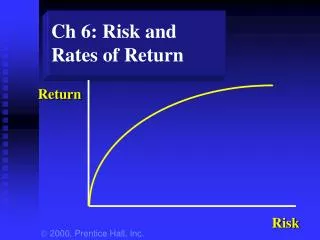
Ch 6.Risk, Return and the CAPM. Goals:. To understand return and risk To understand portfolio To understand diversifiable risks and market (systematic) risks To understand CAPM. 1.Investment returns. Dollar return = amount received –amount invested Problems: Scale effect

E N D
Goals: • To understand return and risk • To understand portfolio • To understand diversifiable risks and market (systematic) risks • To understand CAPM
1.Investment returns • Dollar return = amount received –amount invested Problems: • Scale effect • Times spent or holding period • Rate of return = (amount received – amount invested)/amount invested
2. Stand alone risk • Risk: the chance that some unfavorable event will occur. It is measured by variance or standard deviation – distance from the average. (Stand-alone risk: the risk an investor would face if he or she only held one asset) Ex) Historical return and risk
No investment will be undertaken unless the expected rate of return is high enough to compensate the investor for the perceived risk • To deal with unknown futures, a probability will be applied.
1) Probability distributions • Probability is the chance that the event will occur. • Probability distribution: A listing of all possible outcomes or events with a probability assigned to each outcome. • Discrete & Continuous probability distribution • 68.26% of probability that actual return will be within a mean + or – 1 *standard deviation. • 95.46% of probability that actual return will be within a mean + or – 2 *standard deviation • 99.74% of probability that actual return will be within a mean + or – 3 *standard deviation
Ex) State Probability (P) S B Strong 0.25 0.3 0.2 Normal 0.5 0.15 0.30 Weak 0.25 0.00 -0.10 2) Expected Rates of Returns and Risks: Stand-alone • Expected return
E(ks) = 0.3*0.25+0.15*0.5+0.00*0.25=0.15 • E(kB) = 0.175 • (2) Variance: risk measurement • The tighter the probability distribution, the more likely it is that the actual return will be close to the expected value. Thus the tighter the probability distribution, the lower the risk assigned. It is measured by variance
How to calculate? Standard Deviation
(3) The coefficient of variation: standardized measure of the risk per unit of return. It provides a more meaningful basis for comparison • CV= • CVs=0.10661/0.15 =0.707
(4) Risk Aversion and Required Returns • Risk Aversion: Investors dislike risk and require the higher rate return as an inducement to buy riskier securities. It is commonly assumed in finance. • Therefore, if other things held constant, the higher a security’s risk, the lower its price and the higher its required (expected) returns.
3) Portfolios: Return and Risks Portfolios: combination of assets or securities to minimize total risks and to improve returns (1) Portfolio Returns: Simply the weighted average of the expected returns on individual assets in the portfolio
Ex) using the previous example with an assumption that weights for S and B are 40% and 60%. Expected returns = 0.4(0.15)+0.6(0.175)=0.165
Realized Rate of Return (k bar): • The return actually earned during some past period. It differs from the expected returns (2) Risks • Covariance: measurement of the degree which two assets covary • Correlation coefficient: Standardization of covariance
In our example, • Ws=0.4 WB=0.6 • rSB=0.6469 σs=0.1061 σB=0.1639 • Portfolio risk is 0.016875
Lessons from Portfolio variance calculation • (1) If the numbers of securities composing a portfolio increase, the number of covariance will be greater than number of variances. Thus, the variance of well diversified portfolio reflects the covariance. • (2) If the correlation is less than 1, the covariance will reduce, leading to lower portfolio risks. Diversification effects • (3) If the correlation is 1, the covariance will increase to the maximum value
(4) If the correlation is -1, then the variance will reduce to the minimum value. Diversification effects (5) In reality, securities’ correlations are between 0 and 1. 4) Diversifiable Risk and Market Risk Systematic risk Unsystematic risk Total Risk = Market risk + Firm specific risk Undiversifiable risk Diversifiable risk Nondiversifiable risk
Diversifiable risk: That part of a security’s risk associated with random events, diversified away • Market risk: The part of a security’s risk that can not be eliminated by diversification • If the diversifiable risks can be diversified away, investors are mainly concerned about the systematic (un-diversifiable) risks. They may consider the systematic risk in individual stocks or contribution to risks of well diversified portfolio to be risks compensated.
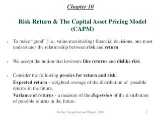
The systematic risk is a market risk inherent in market • 4) The concept of beta • How to measure the systematic risk? • It can be measured by the degree to which a given stock tends to move up or down with the market (stock market). It is called “beta”
Three meanings of beta • to changes in the return of the market portfolio. [the comovement of an asset i's return (price) to the market portfolio's return (price)] • beta is a measure of the undiversifiable (market, systematic) risk of the asset i.
Graphically, it is a slop of a line in the scatter plot composed of market returns and individual stock returns • Beta of a portfolio 5) CAPM (Capital Asset Pricing Model) Based on the beta estimate, we are able to come up with CAPM that will estimate a required rate of return in individual stock.
CAPM: • = risk free rate + market risk premium*beta • kRF: risk free rate • kM: market return Here market risk premium (RPM) is the extra rate of return that investors require to invest in the stock market rather than purchase risk-free securities. It is determined by the degree of risk aversion that investors have on average. • Risk premium (RPi) for stock i = market risk premium*beta
Ex) Currently, T-bill and S&P 500 are offering 3% and 5%. F503 stocks’ beta is 0.7. Required rate of return = 0.03+0.7(0.05-0.03)
SML (security market line): • Equilibrium relationship between the expected returns and the systematic risk of assets (individual stocks or portfolios). • Graphical description of CAPM. • Underpriced: when an asset lies above the SML. Then demand will increase and price will increase, leading the current return to a required return on SML (CAPM).
ri (%) . Alta Market . . rM = 15 rRF = 8 . Am. Foam T-bills . Repo Risk, bi -1 0 1 2
Overpriced: when an asset lies below the SML. Then demand will decrease and price will decrease, leading the current return to a required return on SML (CAPM). • Therefore, in equilibrium, all assets lies on the SML. • 6) Impacts of Inflation. • It will not change market risk premium but increase risk free rate, shifting SML upward
Thus, it will increase a required rate of return from CAPM • 7) Impact of risk aversion. • The slope of SML reflects the extent to which investors are averse to risk. The steeper the slope of the line, the greater the average investor’s risk aversion. • The increasing risk aversion will increase market premium but not change risk free rates
SML rotates counterclockwise. • Equilibrium required rate of return according to the CAPM increases for assets with positive . • Equilibrium required rate of return according to the CAPM decreases for assets with negative . • 8) Impact of changing betas. • Without changing risk free rate and slop of SML, it will increase a required rate of return
9) Form of the Efficient Markets Hypothesis • - weak form: all past information is fully reflected in current market price. E.g) technical analysis • - semi-strong form: current stock price reflects all publicly available information. E.g) • - strong form
10) Empirical tests: joint test of the EMH and an asset pricing model. Whether a certain strategy can beat the market. • Most studies showed that the stock market is highly efficient in the weak form, with two exceptions – long term reversals and short term momentum. Strategies based on reversal and momentum tend to generate an excess return over a return from CAPM. But it is small when transaction cost is considered. • The stock market is reasonable efficient in the semi-strong form. It is difficult to use public information to generate consistent greater returns than those predicted by CAPM. But two exceptions: small size and high book to market ratio. Stocks with these traits tend to generate a greater return than that predicted by CAPM.
11) Behavior Finance • We experienced bubbles in the market. But there was no clear explanation why. Factor models could not explain these bubbles. Behavior finance based on human psychology, however, offers possible explanations: overconfidence, anchoring bias, and herding. • (1) Overconfidence in part stems from two other biases: self attribution and hindsight bias. • - self attribution: people’s tendency to ascribe any success to their own talents while blaming failure on bad luck. • - hindsight: tendency of people to believe they can predict the future than they actually can. • (2) Anchoring bias: tendency of people to rely too much on recent events when predicting the future.
(3) Herding behavior: tendency of investors emulate other successful investors and chase asset classes (eg. Smart money) which are doing well. • Additional one: Loss aversion. • It means that human tends to show a different attitude, depending on receiving or paying money. When receiving money, people want to have certainty. But when they need to pay, they want to take a chance. • E.g) $500 sure or $1000 on the face of a coin and nothing on the tail of the coin. If you receive money, you may want $500. But if you have to pay, you may want to go for the coin.