Download
1 / 45
450 likes | 552 Vues
Gene Recognition. Credits for slides: Serafim Batzoglou Marina Alexandersson Lior Pachter Serge Saxonov. DNA. transcription. RNA. translation. Protein. The Central Dogma. CCTGAGCCAACTATTGATGAA. CCU GAG CCA ACU AUU GAU GAA. P E P T I D E. Gene structure. intron1. intron2. exon2.

E N D
Gene Recognition Credits for slides: Serafim Batzoglou Marina Alexandersson Lior Pachter Serge Saxonov
DNA transcription RNA translation Protein The Central Dogma CCTGAGCCAACTATTGATGAA CCUGAGCCAACUAUUGAUGAA PEPTIDE
Gene structure intron1 intron2 exon2 exon3 exon1 transcription splicing translation Codon: A triplet of nucleotides that is converted to one amino acid exon = protein-coding intron = non-coding
Locating Genes • We have a genome sequence, maybe with related genomes aligned to it…where are the genes? • Yeast genome is about 70% protein coding • About 6000 genes • Human genome is about 1.5% protein coding • About 22,000 genes
Stop codon TAG/TGA/TAA Start codon ATG Finding Genes in Yeast Coding Intergenic Intergenic 5’ 3’ Mean coding length about 1500bp (500 codons) Transcript
Finding Genes in Yeast • ORF Scanning • Look for long open reading frames (ORFs) • ORFs start with ATG and contain no in-frame stop codons • Long ORFs unlikely to occur by chance (i.e., they are probably genes)
Finding Genes in Yeast Yeast ORF distribution
Stop codon TAG/TGA/TAA Start codon ATG Introns: The Bane of ORF Scanning Intergenic Intergenic Intron 5’ Exon Exon Intron Exon 3’ Splice sites Transcript
Introns: The Bane of ORF Scanning • Drosophila: • 3.4 introns per gene on average • mean intron length 475, mean exon length 397 • Human: • 8.8 introns per gene on average • mean intron length 4400, mean exon length 165 • ORF scanning is defeated
Now What? • We need to use more information to help recognize genes • Regular structure • Exon/intron lengths • Nucleotide composition • Biological signals • Start codon, stop codon, splice sites • Patterns of conservation
Regular Gene Structure • Protein coding region starts with ATG, ends with TAA/TAG/TGA • Exons alternate with introns • Introns start with GT/GC, end with AG • Each exon has a reading frame determined by the codon position at the end of the last exon
Next Exon: Frame 0 Next Exon: Frame 1
Nucleotide Composition • Base composition in exons is characteristic due to the genetic code Amino Acid SLCDNA Codons Isoleucine I ATT, ATC, ATA Leucine L CTT, CTC, CTA, CTG, TTA, TTG Valine V GTT, GTC, GTA, GTG Phenylalanine F TTT, TTC Methionine M ATG Cysteine C TGT, TGC Alanine A GCT, GCC, GCA, GCG Glycine G GGT, GGC, GGA, GGG Proline P CCT, CCC, CCA, CCG Threonine T ACT, ACC, ACA, ACG Serine S TCT, TCC, TCA, TCG, AGT, AGC Tyrosine Y TAT, TAC Tryptophan W TGG Glutamine Q CAA, CAG Asparagine N AAT, AAC Histidine H CAT, CAC Glutamic acid E GAA, GAG Aspartic acid D GAT, GAC Lysine K AAA, AAG Arginine R CGT, CGC, CGA, CGG, AGA, AGG
Biological Signals • How does the cell recognize start/stop codons and splice sites? • In part, from characteristic base composition • Donor site (start of intron) is recognized by a section of U1 snRNA U1 snRNA: GUCCAUUCA Donor site consensus: MAGGTRAGT M means “A or C”, R means “A or G”
atg caggtg ggtgag cagatg ggtgag cagttg ggtgag caggcc ggtgag tga
Donor site 5’ 3’ Splice Sites Position % -8 … -2 -1 0 1 2 … 17 A 26 … 60 9 0 0 54 … 21 C 26 … 15 5 0 1 2 … 27 G 25 … 12 78 100 0 41 … 27 T 23 … 13 8 0 99 3 … 25
Splice Sites (http://www-lmmb.ncifcrf.gov/~toms/sequencelogo.html)
Splice Sites • WMM: weight matrix model = PSSM (Staden 1984) • WAM: weight array model = 1st order Markov (Zhang & Marr 1993) • MDD: maximal dependence decomposition (Burge & Karlin 1997) • Decision-tree algorithm to take pairwise dependencies into account • For each position I, calculate Si = ji2(Ci, Xj) • Choose i* such that Si* is maximal and partition into two subsets, until • No significant dependencies left, or • Not enough sequences in subset • Train separate WMM models for each subset G5G-1 G5G-1 A2 G5G-1 A2U6 G5 All donor splice sites not G5 G5 not G-1 G5G-1 not A2 G5G-1A2 not U6
Patterns of Conservation • Functional sequences are much more conserved than nonfunctional sequences • Signal sequences show compensatory mutations • If one position mutates away from consensus, often a different one will mutate to consensus • Coding sequence shows three-periodic pattern of conservation
Three Periodicity • Most amino acids can be coded for by more than one DNA triplet • Usually, the degeneracy is in the last position Human CCTGTT (Proline, Valine) Mouse CCAGTC (Proline, Valine) Rat CCAGTC (Proline, Valine) Dog CCGGTA (Proline, Valine) Chicken CCCGTG (Proline, Valine)
Intron Exon Exon Intron Intergenic Exon Intergenic Hidden Markov Models for Gene Finding First Exon State Intron State Intergene State GTCAGATGAGCAAAGTAGACACTCCAGTAACGCGGTGAGTACATTAA
Intron Exon Exon Intron Intergenic Exon Intergenic Hidden Markov Models for Gene Finding First Exon State Intron State Intergene State GTCAGATGAGCAAAGTAGACACTCCAGTAACGCGGTGAGTACATTAA
GENSCAN • Burge and Karlin, Stanford, 1997 • Before The Human Genome Project • No alignments available • Estimated human gene count was 100,000 • Explicit state duration HMM (with tricks) • Intergenic and intronic regions have geometric length distribution • Exons are only possible when correct flanking sequences are present
GENSCAN • Output probabilities for NC and CDS depend on previous 5 bases (5th-order) • P(Xi | Xi-1, Xi-2, Xi-3, Xi-4, Xi-5) • Each CDS frame has its own model • WAM models for start/stop codons and acceptor sites • MDD model for donor sites • Separate parameters for regions of different GC content
GENSCAN Performance • First program to do well on realistic sequences • Long, multiple genes in both orientations • Pretty good sensitivity, poor specificity • 70% exon Sn, 40% exon Sp • Not enough exons per gene • Was the best gene predictor for about 4 years
TWINSCAN • Korf, Flicek, Duan, Brent, Washington University in St. Louis, 2001 • Uses an informant sequence to help predict genes • For human, informant is normally mouse • Informant sequence consists of three characters • Match: | • Mismatch: : • Unaligned: . • Informant sequence assumed independent of target sequence
The TWINSCAN Model • Just like GENSCAN, except adds models for conservation sequence • 5th-order models for CDS and NC, 2nd-order models for start and stop codons and splice sites • One CDS model for all frames • Many informants tried, but mouse seems to be at the “sweet spot”
TWINSCAN Performance • Slightly more sensitive than GENSCAN, much more specific • Exon sensitivity/specificity about 75% • Much better at the gene level • Most genes are mostly right, about 25% exactly right • Was the best gene predictor for about 4 years
N-SCAN • Gross and Brent, Washington University in St. Louis, 2005 • If one informant sequence is good, let’s try more! • Also several other improvements on TWINSCAN
N-SCAN Improvements • Multiple informants • Richer models of sequence evolution • Frame-specific CDS conservation model • Conserved noncoding sequence model • 5’ UTR structure model
HMM Outputs • GENSCAN • TWINSCAN • N-SCAN Target GGTGAGGTGACCAAGAACGTGTTGACAGTA Target GGTGAGGTGACCAAGAACGTGTTGACAGTA Conservation |||:||:||:|||||:||||||||...... sequence Target GGTGAGGTGACCAAGAACGTGTTGACAGTA Informant1 GGTCAGC___CCAAGAACGTGTAG...... Informant2 GATCAGC___CCAAGAACGTGTAG...... Informant3 GGTGAGCTGACCAAGATCGTGTTGACACAA ...
Homology-Based Gene Prediction • Idea: Try to predict a gene in one organism using a known orthologous gene or protein from another organism • Genewise • Protein homology • Projector • Gene structure homology • Very accurate if (and only if??) homology is high
Evaluating Performance • Three main levels of performance: gene, exon, nucleotide • Two measures of performance: • Sensitivity: what fraction of the true features did we predict correctly? • Specificity: what fraction of our predicted features were correct? • Testing standard is whole-genome prediction • Predicting on single-gene sequences is easier and less interesting
The Future • Many new genomes being sequenced—they will need annotations! • Current experimental “shotgun” methods not enough • However, cheap targeted experiments are available to verify predicted genes • Promising directions in gene prediction: • Conditional random fields • Multiple informants—can we actually get them to work???