Download
1 / 43
440 likes | 675 Vues
Three main points to be covered. Nature, weakness, and (sometime) strength of studies using group-level observations Cohort study as gold standard and its assumptions and limitations Concept of the study base linking case-control design to the cohort design.

E N D
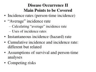
Three main points to be covered • Nature, weakness, and (sometime) strength of studies using group-level observations • Cohort study as gold standard and its assumptions and limitations • Concept of the study base linking case-control design to the cohort design
Studies making observations on groups of individuals vs. individuals • Studies using group level data are usually called ecological studies • Two main points about ecological studies • Weak design for identifying cause and effect associations because of ecological fallacy • In some study situations group-level measures may actually provide better inference than individual-level measures
Example from Szklo and Nieto of grouped data from cohorts in the Seven Countries Study
Ecological Fallacy • Cannot tell whether the predictor and the outcome are related at the individual level • In this example: cannot tell whether the individuals in the cohorts eating less saturated fat are the individuals who are experiencing a higher rate of heart disease • Sometimes called confounding at the group level
Confounding in group data • If no ecological fallacy, still left with possible confounding: some third variable really causing the increase in cancer and also related to number of births • Difficult to control for because measures may not be available • Even if data available, don’t know relationship of confounding variable to other two variables at individual level
Example of the potential strength of measures at group level: Effect of Floods in Bangladesh in 1988 on Children • Children 2 - 9 years samples 6 months before flood and 5 months after • Outcomes: Enuresis and aggressive behavior • Individual level predictor: individual danger of drowning • No association seen at individual level • At group level, before and after flood comparison showed significant difference
Situations where group level variables may be better • Exposures without much within group variability (salt consumption in U.S.) • Herd immunity in studying infectious disease (vaccination levels may be more informative than individual behavior) • Exposures that have powerful effects at group level (Bangladesh flood example)
Conclusions on Ecological Studies • As text emphasizes, common view that they are only hypothesis-generating is inadequate • Weakest design for establishing causality but has a role because inexpensive and easy to do • For some situations and kinds of data may actually be superior • Some variables can only be measured at group level (policies and laws, environment)
Cohort Study Design • Gold standard because exposure/risk factor is observed before the outcome occurs • Randomized trial is a cohort design in which the exposure is assigned rather than observed • Other study designs can be understood by the way in which they sample the experience of a cohort
Cohort study design censored observations = losses to follow-up Minimum loss to follow-up (1%)
Time of Cohort Follow-up vs. Time when measurements made • Concurrent cohorts give most control because measurements are made at the same time as cohort assembly and follow-up (most texts call these prospective cohorts) • Non-concurrent cohorts rely on obtaining measurements made in the past (most texts call these retrospective cohorts) • Mixed cohorts obtain some measures made in the past and rest at same time as follow-up
Selecting a non-concurrent cohort from a current administrative data base • Not a cohort study if you sample persons currently in the data base in order to insure retrospective data from past years • cross-sectional sample • no loss to follow-up by definition • Must sample individuals from some baseline in the past in the data base • ascertain outcome, losses to follow-up from that time forward
Non-concurrent cohort study cannot be defined by presence at end of follow-up This is the cohort Not the cohort
Main Threat to Validity of a Cohort Study • Subjects lost during follow-up • Goal is to retain everyone but number of losses is less important than characteristics of those leaving • How are losses related to outcome and risk factor?
Subjects lost during follow-up • If losses are random, only power is affected • If disease incidence is important question, losses will bias results if related to outcome • If association of risk factor to disease is focus, losses will bias results only if they are related to both outcome and the risk factor • If losses introduce bias in the outcome, the censoring is called informative censoring
Crucial issue is who is leaving cohort: what bias do the censored observations introduce? censored observations = losses to follow-up
Case Control Design: Concept of the Study Base • Study Base = the population that gave rise to the cases (Szklo and Nieto call it the “reference population”) • Key concept that shows the link between case-control design and cohort design • Case-control design using the study base concept is most easily understood in the setting of a cohort study
Nested Case-Control Study within a Cohort Study Study Base = Cohort Controls Sampled each time a Case is diagnosed = Incidence Density
Nested Case-control Study • In text example, 4 cases occur at 4 different points in time giving rise to 4 risk sets of cases and controls • Controls for each case are selected at random in each risk set from cohort subjects under follow-up at the time • It follows from the random selection, that a control can later become a case • Results can be just as valid as using entire cohort; gives unbiased estimate of rate ratio
Definition of a Primary Study Base • Primary Study Base = population that gives rise to cases that can be defined before cases appear by a geographical area or some other identifiable entity like a health delivery system
Examples of Primary Study Bases • Residents of San Francisco during 2001 • Members of the Kaiser Permanente system in the Bay Area during 2001 • Military personnel stationed at California bases during 2001
Example of Case-Control Incidence Density Sampling in a Primary Study Base • Use cancer registry covering San Francisco County to identify all new cases of glioma during a defined time period • At time each new glioma case is reported, randomly sample two controls from current residents of San Francisco
Incidence Density Sampling in a Primary Study Base (e.g., San Francisco County) Primary Study Base New residents Nested case-control in an open cohort with new subjects entering
Case-Control Incidence Density Sampling in a Primary Study Base • Same as nested case-control sampling in a cohort study with exception that in-migration of new persons requires one additional assumption • Just as losses to the study base should not bias the results, additions to the study base should not introduce bias
Primary vs. Secondary Base • Main problem with a primary base is often ascertainment of all cases • Main problem with a secondary base is the definition of the base
Case-Based Case-Control Study: The Secondary Study Base • Secondary Study Base = population that gave rise to cases, identified after cases diagnosed; those persons who would have been among the cases if they had developed the disease during the time period of study • Start with a cases and then attempt to identify hypothetical cohort that gave rise to them
Case-Based Case Control Studies and the Secondary Study Base • Source of cases is often one or more hospitals or other medical facilities • Problem is identifying the population who would come to those institutions if they were diagnosed with the disease • Careful consideration has to be given to factors causing someone to show up at that institution with that diagnosis
Case-control study starting with a sample of cases and identifying secondary study base Secondary study base Sampling can be incidence density just as in primary study base
Case-Based Case Control Studies • Example: glioma cases seen at UCSF • Difficult because referrals come from many areas • One possible control group might be UCSF patients with a different neurologic disease • Patients from a similar tertiary referral clinic are another possible control group
Text example of case-based case-control design shows sampling prevalent controls Secondary Study Base
Case-based design using prevalent cases: essentially same as cross-sectional design
Example of case-based design using prevalent cases • Sampling glioma patients under treatment in a hospital during study period • Poor survival so patients in treatment will over-represent those who live longest • Nature of bias variable and not predictable
Study base and case-control design Critical point of case-control design is that the cases need to consist of all, or a random sample, of subjects in the base experiencing the outcome and the controls need to consist of a sample of the base that can be used to estimate the exposure distribution in the base
Summary Points • Ecological studies weak in showing cause but have some valuable features • Nature, not the size, of losses to follow-up crucial in cohort studies • Key to case-control design is specifying and sampling the study base • Case-control results can be as valid as cohort results if study properly designed and measurements made without bias
Does Pregnancy Protect Against Ovarian Cancer?(Beral, Fraser, and Chilvers, Lancet, 1978) Compared changes in average number of children vs. ovarian CA mortality rates over time: Average family size of women born in each 5-year interval between 1861 and 1931 in England and the U.S. was compared to the ovarian CA mortality rates (standardized) for women of those 5-year generations
Beral et al., Lancet 1978 r = - 0.97
Strengthening Ecological Associations withmultiple group-level comparisons: Five additional types of group data were used • Across Countries: Average family size in 20 countries for women born around 1901 vs. ovarian CA mortality • By marital status and social class: Ovarian CA mortality rates among women 55-64 in England and Wales by marital status and social class • By religion: Incidence follows family size for Catholic, Protestant, and Jewish women in N.Y. state • By ethnic group: U.S. blacks and Am. Ind. vs. whites • Among immigrants: Rates changed with family size
Ovarian Cancer versus average family size in 20 countries Beral et al., Lancet 1978 r = - 0.75
Example of effect of losses to follow-up in a cohort study: 100 subjects, 30 with risk factor (RF) and 70 without 1/3 (10/30) with RF develop disease within a year 1/10 (7/70) without RF develop disease within a year With no losses to follow-up in one year: Disease incidence = 17/100 = 17% in one year RR = 10/30 / 7/70 = 3.33
Example: 100 subjects, 30 with risk factor (RF) and 70 without Losses to follow-up related to disease but not to RF: 9 of 30 (30%) with RF and 10 of 70 (14%) without RF lost to follow-up in one year but risk in each group remains 1/3 and 1/10 Disease incidence = 13/100 = 13% in one year Relative Risk = 7/21 / 6/60 = 3.33 Incidence is changed but Relative Risk is not
Example: 100 subjects, 30 with risk factor (RF) and 70 without Losses to follow-up related to both RF and disease: 9 of 30 (30%) with RF and 10 of 70 (14%) without RF lost to follow-up in one year, and risk in each group is changed. Risk with RF is now 1/4 and without RF is 1/6. Disease incidence = 15/100 = 15% in one year Relative Risk = 5/21 / 10/60 = 1.43 Both Relative Risk and Incidence are changed