Download
1 / 31
310 likes | 315 Vues
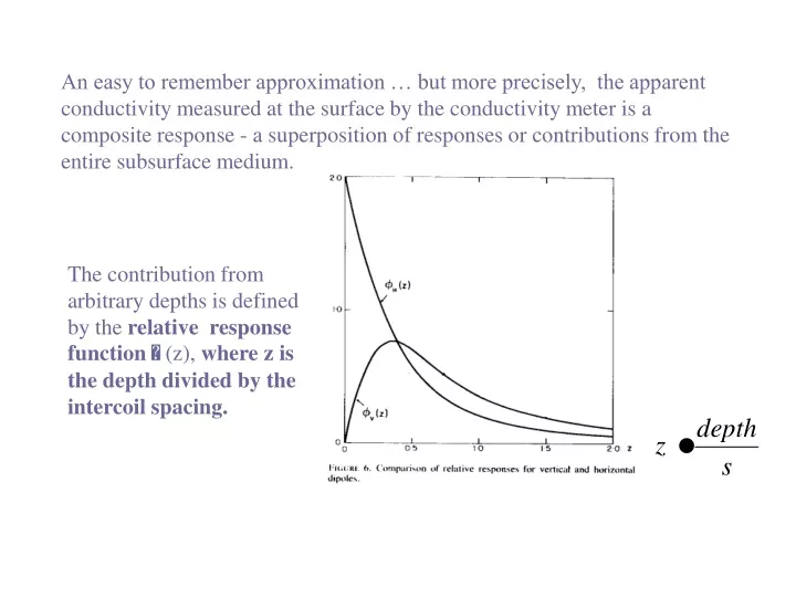
An easy to remember approximation … but more precisely, the apparent conductivity measured at the surface by the conductivity meter is a composite response - a superposition of responses or contributions from the entire subsurface medium.

E N D
An easy to remember approximation … but more precisely, the apparent conductivity measured at the surface by the conductivity meter is a composite response - a superposition of responses or contributions from the entire subsurface medium. The contribution from arbitrary depths is defined by the relative response function (z), where z is the depth divided by the intercoil spacing.
Note that the relative response function for the horizontal dipole h is much more sensitive to near-surface conductivity variations and that its response or sensitivity drops off rapidly with depth Vertical dipole interaction has no sensitivity to surface conductivity, reaches peak sensitivity at z ~0.5, and is more sensitive to conductivity at greater depths than is the horizontal dipole. For next time continue your reading of McNeill and develop a general appreciation of the relative and cumulative response functions.
Constant conductivity The contribution of this thin layer to the overall ground conductivity is proportional to the value of the relative response function at that depth.
Z1 Z2 The contribution of a layer to the overall ground conductivity is proportional to the area under the relative response function over the range of depths (Z2 -Z1) spanned by that layer.
As you might expect, the contribution to ground conductivity of a layer of constant conductivity that extends significant distances beneath the surface (i.e. homogenous half-space) is proportional to the total area under the relative response function.
So in general the contribution of several layers to the overall ground conductivity will be in proportion to the areas under the relative response function spanned by each layer.
You all will recognize these area diagrams as integrals. The contribution of a given layer to the overall ground conductivity at the surface above it is proportional to the integral of the relative response function over the range of depths spanned by the layer.
McNeill introduces another function, R(z) - the cumulativeresponse function - which he uses to compute the ground conductivity from a given distribution of conductivity layers beneath the surface. The following diagrams are intended to help you visualize the relationship between R(z) and (z).
Each point on the RV(z) curve represents the area under the V(z) curve from z to .
Consider one additional integral - How would you express this integral as a difference of cumulative response functions?
According to our earlier reasoning - the contribution of a single conductivity layer to the measured ground (or terrain) conductivity is proportional to the area under the relative response function. The apparent conductivity measured by the terrain conductivity meter at the surface is the sum total of the contributions from all layers. We know that each of the areas under the relative response curve can be expressed as a difference between cumulative response functions
Let’s consider the following problem, which is taken directly from McNeill’s technical report (TN6).
Mathematical formulation - Compare this result to that of McNeill’s (see page 8 TN6).
In this relationship ais the apparent conductivity measured by the conductivity meter. The dependence of the apparent conductivity on intercoil spacing is imbedded in the values of z. Z for a 10 meter intercoil spacing will be different from z for the 20 meter intercoil spacing. The above equation is written in general form and applies to either the horizontal or vertical dipole configuration.
In the appendix of McNeill (today’s handout), he notes that the assumption of low induction number yields simple algebraic expressions for the relative and cumulative response functions. We can use these relationships to compute specific values of R for given z’s.
The simple algebraic expressions for RV(z) and RH(z) make it easy for us to compute the terms in the problem McNeill gives us. In that problem z1 is given as 0.5 and z2 as 1 and 1.5 Assuming a vertical dipole orientation RV(z=0.5) ~ 0.71 RV(z=1.0) ~ 0.45 RV(z=1.5) ~ 0.32
Z1 = 0.5 1=20 mmhos/m 2=2 mmhos/m Z2 = 1 and 1.5 3=20 mmhos/m Substituting in the following for the case where Z2=1.
Mine spoil surface AMD contamination zone ~10ft ~60ft Pit Floor Here’s a problem for you to work through before our next class. A terrain conductivity survey is planned using the EM31 meter (3.66 m (or 12 foot) intercoil spacing). Our hypothetical survey was conducted over a mine spoil to locate migration pathways within the spoil through which acidic mine drainage as well as neutralizing treatment are being transported. Scattered borehole data across the spoil suggest that these paths are approximately 10 feet thick and several meters in width. Borehole resistivity logs indicate that areas of the spoil surrounding these conduits have low conductivity averaging about 4mmhos/m. The bedrock or pavement at the base of the spoil also has a conductivity of approximately 4mmhos/m. Depth to the pavement in the area of the proposed survey is approximately 60 feet. Conductivity of the AMD transport channels is estimated to be approximately 100mmhos/m.
A. Evaluate the possibility that the EM31 will be able to detect high conductivity transport zones with depth-to-top of 30feet. Evaluate only for the vertical dipole mode. It may help to draw a cross section.
How many different conductivity layers will you actually have to consider? Does it matter whether d (depth) and s (intercoil spacing) are in feet or meters? Set up your equation following the example presented by McNeill and reviewed in class, and solve for the apparent conductivity recorded by the EM31 over this area of the spoil. Bring your work in and be prepared to discuss it at the beginning of the next class. Note - a table of R values are presented on the following page.
Z RV RH .000 1.000000 1.000000 .200 .9284767 .6770329 .400 .7808688 .4806249 .600 .6401844 .3620499 .800 .5299989 .2867962 1.000 .4472136 .2360680 1.200 .3846154 .2000000 1.400 .3363364 .1732137 1.600 .2982750 .1526108 1.800 .2676438 .1363084 2.000 .2425356 .1231055 2.200 .2216211 .1122055 2.400 .2039542 .1030602 2.600 .1888474 .0952811 2.800 .1757906 .0885849 3.000 .1643990 .0827627 3.200 .1543768 .0776539 3.400 .1454940 .0731363 3.600 .1375683 .0691128 3.800 .1304545 .0655074 4.000 .1240347 .0622578 4.200 .1182129 .0593147 4.400 .1129097 .0566359 4.600 .1080592 .0541887 4.800 .1036061 .0519428 5.000 .0995037 .0498762 5.200 .0957124 .0479660 5.400 .0921982 .0461979 5.600 .0889320 .0445547 5.800 .0858884 .0430231