Download
1 / 43

E N D
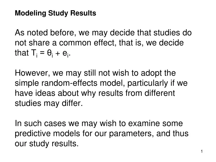
Modeling Study ResultsAs noted before, we may decide that studies do not share a common effect, that is, we decide that Ti = θi + ei.However, we may still not wish to adopt the simple random-effects model, particularly if we have ideas about why results from different studies may differ. In such cases we may wish to examine some predictive models for our parameters, and thus our study results.
Predictive or Explanatory Models We will consider the regression model θi = 0 + 1 X1i + ... + p XpiWe’ll also examine an ANOVA-like model, where the subscript j shows that study i is from the jth group or category of studies θji = θj for study i in group j Both analyses will be weighted using w or another weight.
Mixed Effects Models If each population effect differs, and Ti = i + ei we may want to model or explain the variation in the population effects. For example we may have i = b0 + b1X1i + u’i Substituting, we have Ti =b0 + b1X1i + u’i + ei Observed Effect predicted + Unexplained between- + Sampling effect from X value studies variation error
Going back to the model for Ti, we see that for the regression model Ti = 0 + 1 X1i + ... + p Xpi + eiand for the ANOVA model Tji = θj + ejiFor both models we will have tests of significance and tests and estimates of slopes, means, etc. Also we’ll have tests of model specification that tell us whether we have explained all between studies differences.
For instance, for the expectancy studies, we can analyze weeks before the expectancy induction occurred, both as a categorical factor, and as a regression predictor: Ti = 0 + 1 weeksi +ei .For the ANOVA-like model we can group studies by weeks: 0 weeks exposure 1 week exposure 2 weeks exposure 3 or more weeks of exposure
A key difference between what we do for meta-analysis and standard OLS regression and ANOVA is that meta-analysis data typically violate the assumption of homoscedasticity, because study sizes differ and Vi values are not equal. For example, in the meta-analysis regression Ti = 0 + 1 X1i + ... + p Xpi + eiwe know that v(ei) can be computed and is a function of ni. If the ni’s vary, we won’t have homoskedasticity.
Therefore, weighted analogues to the typical analyses are needed. Our models show the only source of variation to be sampling error (the ei terms). We begin by using the weights used before: wi = 1/vi .These are our fixed effects weights, and shortly we will have a third set of weights as well.
Technically, we use weighted least squares (WLS) regression and weighted ANOVAs. We do not use random-effects weights because we are trying to explain the between-studies differences that the RE model treats as “uncertainty.” Using RE weights gives a very conservative analysis. Later we will learn about mixed models. We use these if our ANOVA or regression analyses do not explain all of the between-studies differences in our data.
Weighted Regression for Meta-analysis (AKA meta-regression)The estimation of regression slopes is done via weighted least squares (WLS) regression.We have a vector of outcomes T = (T1, T2, . . . Tk)’ and a matrix of p predictors, called X Denote the matrix of variances of the outcomes T1, T2, ... Tk as Σ = diag[V1, ... ,Vk ] .
Then the WLS gives us^ = (X’ Σ-1 X)-1 X’ Σ-1 Tthe vector of slopes, and its variance is^ V() = (X’ Σ-1 X)-1Under H0: β = 0, the p slope estimates are normally distributed, so the standard output is not correct.
The printed standard computer output from pull-down menus shows slopes that are correct BUT SEs and t tests that are INCORRECT!!If we use pullodwn menus we must correct the SEs via SE = Printed SE/MSE ^ ^ Also the tests can be computed as z = /SE()or as z = (Printed test ) *MSEBut why do that when we can use SPSS macros to get the right results!
Also we have two tests that tell us about our models: QModel + QResidual = Q2(p)2(k-p-1)2(k-1)In pulldown output we can look at SSModel + SSResidual = SSTotalWe then ask a series of questions.
First we ask ...1. Is QModel significant?If yes, the predictors explain some (or all) of the population variationIf not, we might look for another predictor or try another modelWe’ll look at the expectancy data with “weeks” as our predictor.
The scatterplot shows a somewhat nonlinear relationship with “weeks” as the predictor.Note that the “best fit” line that SPSS plots will not be correct unless all studies are equal in size. This occurs because we need to use a weighted regression and the plotted line is unweighted.
We can make a plot that shows the weight each study gets under the fixed model. The points vary in size. Large circles show the larger studies that have more weight.
The fitted equation is obtained from pull-downs using the regression menu with “w” clicked into the box for the “WLS weight”. The model isdi = 0.158 - 0.013 weeksi + ei SSRegression = QReg = 8.16 is significant with p = 1 df.
The macro from Dave Wilson called MetaReg.sps gives this analysis with proper CIs. Do not use the R2 -- it is too low. ***** Inverse Variance Weighted Regression ***** ***** Fixed Effects Model via OLS ***** ------- Descriptives ------- Mean ES R-Square k .0603 .2278 19.0000 ------- Homogeneity Analysis ------- Q df p Model 8.1609 1.0000 .0043 Residual 27.6645 17.0000 .0490 Total 35.8254 18.0000 .0074 ------- Regression Coefficients ------- B SE -95% CI +95% CI Z P Beta Constant .1584 .0501 .0602 .2566 3.1620 .0016 .0000 weeks -.0132 .0046 -.0223 -.0041 -2.8567 .0043 -.4773
Here’s the regression line from the weighted analysis:di = 0.158 - 0.013 weeksi + ei Clearly the points with the large effects at weeks = 0 are not well explained by this line.
Next we check the specification of the model by asking2. Is QResidual significant?If QResidual is small, then the predictors explain all between-studies differencesIf QResidual is big, then unexplained differences remain and the predictors do not give a full explanation. We may want to explore other predictors or run a mixed model.
The MetaReg output shows that the Q for residual is just significant. Using weeks as a continuous predictor does not quite explain the variation in effects. With one X, the ps for the model and the slope are identical. Just significant. ------- Homogeneity Analysis ------- Q df p Model 8.1609 1.0000 .0043 Residual 27.6645 17.0000 .0490 Total 35.8254 18.0000 .0074 ------- Regression Coefficients ------- B SE -95% CI +95% CI Z P Beta Constant .1584 .0501 .0602 .2566 3.1620 .0016 .0000 weeks -.0132 .0046 -.0223 -.0041 -2.8567 .0043 -.4773
Mixed Regression ModelIf we have not explained all variation it means there is excess uncertainty to account for. That is, our model is Ti =b0 + b1X1i + ei + uꞋi.so we need to estimate the variance of the uꞋi. We do this by using a mixed model. Let’s see what MetaReg tells us about how much uncertainty remains, and how it affects the model.
MetaReg shows that the Q for residual is no longer significant. However, this is not really a legitimate test, so we do not report it. We are more interested in the Model test. Weeks is still significant even with added uncertainty accounted for! ------- Homogeneity Analysis ------- Q df p Model 7.9277 1.0000 .0049 Residual 24.2264 17.0000 .1134 Total 32.1541 18.0000 .0211
MetaReg shows the residual variance as .0048, well below either of the RE variances. The model is Ti = 0.18 - .0146 +ei + uꞋi vs.the (wrong) FE model Ti = 0.16 - .0132 +ei ------- Regression Coefficients ------- B SE -95% CI +95% CI Z P Beta Constant .1773 .0567 .0662 .2884 3.13 .0018 .0000 weeks -.0146 .0052 -.0247 -.0044 -2.82 .0049 -.4965 --- Maximum Likelihood Random Effects Variance Component ---- v = .00485 se(v) = .00888
ANOVA-Like Categorical ModelConsider studies that fall into p a priori groups. Then we have Tji the outcome for study i in group or class j, for i = 1 to kj studies in j = 1 to p groups with k = Σ kjDenote_Tj The estimated average effect in group jθj The true population effect in group j
We ask the question: Do all θj values agree?Our null hypothesis is like that for the between-groups test in ANOVA:H0: θ1 = θ2 = . . . = θpIn words H0 says: All p sets of studies show the same population effects, or, The mean effects in the p groups are equal.
We also ask the question: Do all θji values in the jth group agree?This null hypothesis is like that for the overall Q test, but it is done within each of the p groups. For example, for group 1 we haveH01: θ11 = θ12 = . . . = θ1 k1 = θ1 In words H01 says “All studies in group 1 show the same population effect.”
So for each of the groups (j=1 to p) we test this H0jH0j: θj1 = θj2 = . . . = θj kj = θj For each group we get a Q value within the group (we’ll call it Qwithin j). Then we can get an overall test of within-group homogeneity across the p groups. We get it as Qwithin = Qwithin j
We will partition our total Q into two chi-square tests Q = QBetween + QWithin2(k-1)2(p-1)2(k-p)In standard SPSS pulldown output we’d examine SSTotal = SSBetween + SSWithin Tests differences between the p θj values Tests for remaining variation in results Total homogeneity test
So we have parallel quantities Q = QBetween + QWithin SSTotal = SSBetween + SSWithinQ = SSTotal = All between-studies variation + sampling errorQBetween = SSBetween = Between-groups variation + sampling errorQWithin = SSWithin = Unexplained between-studies differences + sampling error
_Tj is computed similarly, but within group j _ Tj = wji Tji / wji for wji = 1/Vji i iWe can also get variances and SEs for these means (more on this below). QWj is a weighted variance of the effects within group j and QWithin is the sum of those variancesp kj _ _QWithin = wji (Tji - Tj)2 = QWj ~ 2(k-p) j iEach QWj is a chi-square test with df = kj - 1
We ask a series of questions about these tests:1. Is QBetween significant?If yes, the predictor explains some (or all) of the population variationIf not, we decide that the grouping variable that was tested does not explain between-studies differences. We might look for another predictor for ANOVA or try another kind of model. This factor, though, is not useful if Qbetween is not significant.
Example: Teacher expectancy effects Here we’ll look at exposure in terms of number of weeks the teachers had known the students (weekcat in our data). The means appear to be lower with more weeks of exposure. Let us examine the hypothesis of no differences.
We can use a macro called MetaF.sps developed by Dave Wilson. The output from his macro looks like this: The correct p values for the chi-square tests are given. Differences exist between groups. ***** Inverse Variance Weighted Oneway ANOVA ***** ***** Fixed Effects Model via OLS ***** ------- Analog ANOVA table (Homogeneity Q) ------- Q df p Between 20.3788 3.0000 .0001 Within 15.4466 15.0000 .4198 Total 35.8254 18.0000 .0074
Next (if QBetween is significant) we ask 2. Is QWithin significant and are any QWj values significant?If the QWj’s are small and QWithin is small, then the predictor explains all between-studies differences.If a few QWj’s are big and QWithin is small, then the predictor explains most between-studies differences -- outliers may be a possibilityor we may need a mixed model.
The output showed significant between-groups differences and, considering all groups, we do not see heterogeneity within groups (p = .42 which is quite large). The ANOVA model appears to fit perfectly! But let’s check each group. ***** Inverse Variance Weighted Oneway ANOVA ***** ***** Fixed Effects Model via OLS ***** ------- Analog ANOVA table (Homogeneity Q) ------- Q df p Between 20.3788 3.0000 .0001 Within 15.4466 15.0000 .4198 Total 35.8254 18.0000 .0074
------- Q by Group ------- Group Qw df p .0000 6.2140 4.0000 .1837 1.0000 4.9825 2.0000 .0828 2.0000 .4045 2.0000 .8169 3.0000 3.8456 7.0000 .7974 MetaF.sps produces this table: Each line gives a Q for a subset of studies (here for weekcat groups). All p values are above .05, suggesting each subset is homogeneous. If they were not, we would use a mixed model.
The MetaF.sps macro produces a table of means as well. The overall mean does not differ from 0. • Two group means differ from zero (weekcat = 0 and 1) and two do not. ------- Effect Size Results Total ------- Mean ES SE -95%CI +95%CI Z P k Total .0603 .0365 -.0112 .1319 1.6539 .0981 19.00 ------- Effect Size Results by Group ------- Group Mean ES SE -95%CI +95%CI Z P k .0000 .3620 .1099 .1466 .5774 3.2939 .0010 5.00 1.0000 .3516 .1121 .1319 .5712 3.1367 .0017 3.00 2.0000 .0665 .0727 -.0760 .2091 .9147 .3604 3.00 3.0000 -.0630 .0500 -.1611 .0350 -1.2605 .2075 8.00
Contrasts for ANOVA-like ModelsIf we reject H0: θ1 = θ2 = . . . = θp(i.e.,QBetween is significant) or if we have some groups we would like to compare based on a priori hunches, we can use the values of the means (the Tj) to compute contrasts: C = Σ cj Tj where Σ cj = 0.We compute the SE for C, and the test statistic is z = C/SE(C).
The contrasts parallel traditional ANOVA contrasts and can be used, e.g., to compare the mean of the combined TE weekcat groups 0 and 1 to that of groups 2 and 3. The hypothesis tested isH0: (θ0 + θ1)/2 =(θ2 + θ3)/2The contrast is C = (T0 + T1)/2 -(T2 + T3)/2 = Σ cj Tj
If the contrast is C = Σ cj Tj , then SE(C) = Σ c2j Var (Tj)Here SE(C) =Often it is easier to use integer weights so we don’t have fractions in the varianceFor the TE data, we could use integer weights cj of 1 and -1, then C = (T0 + T1) - (T2 + T3)
For our data for the contrast using fractional weightsC = (T0 + T1)/2 -(T2 + T3)/2 = Σ cj Tj = (.362 + .352)/2 - (.067 + -.063)/2 = .357 - .002 = .355 __________________________SE (C) = .012/4 + .013/4 + .005/4 + .002/4 = 0.089
The test of H0 is z = C/SE(C) = .355/.089 = 3.97 so we reject H0: (θ0 + θ1)/2 =(θ2 + θ3)/2It seems that students exposed to teachers for a week or less show significantly larger mean expectancy effects than students with 2 or more weeks exposure.