Download
1 / 27
280 likes | 413 Vues
CLUSTERING Basic Concepts In clustering or unsupervised learning no training data, with class labeling, are available. The goal becomes: Group the data into a number of sensible clusters (groups). This unravels similarities and differences among the available data. Applications:

E N D
CLUSTERING • Basic Concepts In clustering or unsupervised learning no training data, with class labeling, are available. The goal becomes: Group the data into a number ofsensible clusters (groups). This unravels similarities and differences among the available data. • Applications: • Engineering • Bioinformatics • Social Sciences • Medicine • Data and Web Mining • To perform clustering of a data set, a clustering criterionmust first be adopted. Different clustering criteria lead, in general, to different clusters.
Two clusters • Clustering criterion:How mammals beartheir progeny Lizard, sparrow, viper, seagull, gold fish, frog, red mullet Blue shark, sheep, cat, dog Sheep, sparrow, dog, cat, seagull, lizard, frog, viper • Two clusters • Clustering criterion:Existence of lungs Gold fish, red mullet, blue shark • A simple example
Clustering task stages • Feature Selection: Information rich features-Parsimony • Proximity Measure: This quantifies the term similar or dissimilar. • Clustering Criterion: This consists of a cost function or some type of rules. • Clustering Algorithm: This consists of the set of steps followed to reveal the structure, based on the similarity measureand the adopted criterion. • Validation of the results. • Interpretation of the results.
Depending on the similarity measure, the clustering criterion and the clustering algorithm different clusters may result. Subjectivity is a reality to live with from now on. • A simple example: How many clusters?? 2 or 4 ??
Basic application areas for clustering • Data reduction. All data vectors within a cluster are substituted (represented) by the corresponding cluster representative. • Hypothesis generation. • Hypothesis testing. • Prediction based on groups.
Clustering Definitions • Hard Clustering: Each point belongs to a single cluster • Let • An m-clustering R of X, is defined as the partition of X into m sets (clusters), C1, C2,…,Cm, so that In addition, data in Ci are more similar to each other and less similar to the data in the rest of the clusters. Quantifying the terms similar-dissimilar depends on the types of clusters that are expected to underlie the structure of X.
Fuzzy clustering: Each point belongs to all clusters up to some degree. A fuzzy clustering of X into m clusters is characterized by mfunctions
These are known as membership functions. Thus, each xibelongs to any cluster “up to some degree”, depending on the value of
TYPES OF FEATURES • With respect to their domain • Continuous(the domain is a continuous subset of ). • Discrete(the domain is a finite discrete set). • Binaryor dichotomous(the domain consists of two possible values). • With respect to the relative significance of the values they take • Nominal (the values code states, e.g., the sex of an individual). • Ordinal (the values are meaningfully ordered, e.g., the rating of the services of a hotel (poor, good, very good, excellent)). • Interval-scaled (the difference of two values is meaningful but their ratio is meaningless, e.g., temperature). • Ratio-scaled (the ratio of two values is meaningful, e.g., weight).
PROXIMITY MEASURES • Between vectors • Dissimilarity measure(between vectors of X) is a function with the following properties
If in addition (triangular inequality) d is called a metric dissimilarity measure.
Similarity measure(between vectors of X) is a function with the following properties
If in addition s is called a metric similarity measure. • Between sets Let Di X, i=1,…,k and U={D1,…,Dk} A proximity measure on U is a function A dissimilarity measure has to satisfy the relations of dissimilarity measure between vectors, where Di’ ‘s are used in place of x, y(similarly for similarity measures).
PROXIMITY MEASURES BETWEEN VECTORS • Real-valued vectors • Dissimilarity measures (DMs) • Weighted lp metric DMs Interesting instances are obtained for • p=1 (weighted Manhattan norm) • p=2 (weighted Euclidean norm) • p=∞ (d(x,y)=max1ilwi|xi-yi| )
Other measures where bj and ajare the maximum and the minimum values of the j-th feature, among the vectors of X (dependence on the current data set)
Similarity measures • Inner product • Tanimoto measure
Discrete-valued vectors • Let F={0,1,…,k-1} be a set of symbols and X={x1,…,xN} Fl • Let A(x,y)=[aij],i,j=0,1,…,k-1, where aij is the number of places where xhas the i-th symbol and yhas the j-th symbol. NOTE: Several proximity measures can be expressed as combinations of the elements of A(x,y). • Dissimilarity measures: • The Hamming distance (number of places where x and y differ) • The l1 distance
Similarity measures: • Tanimoto measure : where • Measures that exclude a00: • Measures that include a00:
Mixed-valued vectors Someof the coordinatesof the vectors xarerealand the rest arediscrete. Methods for measuring the proximity between two such xi and xj: • Adopt a proximity measure (PM) suitable for real-valued vectors. • Convert the real-valued features to discrete ones and employ a discrete PM. The more general case of mixed-valued vectors: • Here nominal, ordinal, interval-scaled, ratio-scaled features are treated separately.
The similarity function between xi and xj is: In the above definition: • wq=0, if at least one of the q-th coordinates of xi and xj are undefined or both the q-th coordinates are equal to 0. Otherwise wq=1. • If the q-th coordinates are binary, sq(xi,xj)=1 if xiq=xjq=1 and 0 otherwise. • If the q-th coordinates are nominal or ordinal, sq(xi,xj)=1 if xiq=xjqand 0otherwise. • If the q-th coordinates are interval or ratio scaled-valued where rq is the interval where the q-th coordinates of the vectors of the data set X lie.
Fuzzy measures Let x, y[0,1]l. Here the value of the i-th coordinate, xi, of x, is not the outcome of a measuring device. • The closer the coordinate xi is to 1 (0), the more likely the vector xpossesses (does not possess) the i-th characteristic. • As xi approaches 0.5, the certainty about the possession or not of the i-th feature from xdecreases. A possible similarity measure that can quantify the above is: Then
Missing data For some vectors of the data set X, some features values are unknown Ways to face the problem: • Discard all vectors with missing values (not recommended for small data sets) • Find the mean value mi of the available i-th feature values over that data set and substitute the missing i-th feature values with mi. • Define bi=0, if both the i-th featuresxi, yi are available and 1otherwise. Then where (xi,yi) denotes the PM between two scalars xi, yi. • Find the average proximities avg(i) between all feature vectors in X along all components. Then where (xi,yi)=(xi,yi), if both xi and yi are available and avg(i) otherwise.
PROXIMITY FUNCTIONS BETWEEN A VECTOR AND A SET • Let X={x1,x2,…,xN} and C X, x X • All points of C contribute to the definition of (x, C) • Max proximity function • Min proximity function • Average proximity function (nC is the cardinality of C)
A representative(s) of C, rC, contributes to the definition of (x,C) In this case: (x,C)=(x,rC) Typical representatives are: • The mean vector: • The mean center: • The median center: NOTE: Other representatives (e.g., hyperplanes, hyperspheres) are useful in certain applications (e.g., object identification using clustering techniques). wherenC is the cardinality ofC d: a dissimilarity measure
PROXIMITY FUNCTIONS BETWEEN SETS • Let X={x1,…,xN}, Di, Dj X and ni=|Di|, nj=|Dj| • All points of each set contribute to (Di,Dj) • Max proximity function (measure but not metric, only if is a similarity measure) • Min proximity function (measure but not metric, only if is a dissimilarity measure) • Average proximity function (not a measure, even if is a measure)
Each set Di is represented by its representative vector mi • Mean proximity function (it is a measure provided that is a measure): NOTE: Proximity functions between a vector x and a set C may be derived from the above functions if we set Di={x}.
Remarks: • Different choices of proximity functions between sets may lead to totally different clustering results. • Different proximity measures between vectors in the same proximity function between sets may lead to totally different clustering results. • The only way to achieve a proper clustering is • by trial and error and, • taking into account the opinion of an expert in the field of application.