Download
1 / 24
240 likes | 332 Vues
Basic Models of Probability. Instructor: Ron S. Kenett Email: ron@kpa.co.il Course Website: www.kpa.co.il/biostat Course textbook: MODERN INDUSTRIAL STATISTICS, Kenett and Zacks, Duxbury Press, 1998. Course Syllabus. Understanding Variability Variability in Several Dimensions

E N D
Basic Models of Probability Instructor: Ron S. Kenett Email: ron@kpa.co.il Course Website: www.kpa.co.il/biostat Course textbook: MODERN INDUSTRIAL STATISTICS, Kenett and Zacks, Duxbury Press, 1998 (c) 2000, Ron S. Kenett, Ph.D.
Course Syllabus • Understanding Variability • Variability in Several Dimensions • Basic Models of Probability • Sampling for Estimation of Population Quantities • Parametric Statistical Inference • Computer Intensive Techniques • Multiple Linear Regression • Statistical Process Control • Design of Experiments (c) 2000, Ron S. Kenett, Ph.D.
The Paradox of the Chevalier de Mere - 1 Game A Success = at least one “1” (c) 2000, Ron S. Kenett, Ph.D.
The Paradox of the Chevalier de Mere - 2 Game B Success = at least one “1,1” (c) 2000, Ron S. Kenett, Ph.D.
The Paradox of the Chevalier de Mere - 3 Game A Game B P (Success) = P(at least one “1”) P (Success) = P(at least one “1,1”) Experience proved otherwise ! Game A was a better game to play (c) 2000, Ron S. Kenett, Ph.D.
The Paradox of the Chevalier de Mere - 4 The calculations of Pascal and Fermat Game A Game B P (Failure) = P(no “1”) P (Failure) = P(no “1,1”) P (Success) = .518 P (Success) = .491 What went wrong before? (c) 2000, Ron S. Kenett, Ph.D.
P(outcomes add up to “10”) =? To add or to multiply ? (c) 2000, Ron S. Kenett, Ph.D.
1,1 1,2 1,3 1,4 1,5 1,6 2,1 2,2 2,3 2,4 2,5 2,6 3,1 3,2 3,2 3,4 3,5 3,6 4,1 4,2 4,3 4,4 4,5 4,6 5,1 5,2 5,3 5,4 5,5 5,6 6,1 6,2 6,3 6,4 6,5 6,6 P(outcomes add up to “10”) 36 / 3 = (c) 2000, Ron S. Kenett, Ph.D.
Mutually Exclusive Events Two events are mutually exclusive (or disjoint) if it is impossible for them to occur together. If two events are mutually exclusive, they cannot be independent and vice versa. Example: A subject in a study cannot be both male and female, nor can they be aged 20 and 30. A subject could however be both male and 20, both female and 30. (c) 2000, Ron S. Kenett, Ph.D.
Independent Events Two events are independent if the occurrence of one of the events gives us no information about whether or not the other event will occur; that is, the events have no influence on each other. If two events are independent then they cannot be mutually exclusive (disjoint) and vice versa. (c) 2000, Ron S. Kenett, Ph.D.
Example Suppose that a man and a woman each have a pack of 52 playing cards. Each draws a card from his/her pack. Find the probability that they each draw the ace of clubs. We define the events A = 'the man draws the ace of clubs' B = 'the woman draws the ace of clubs' Clearly events A and B are independent so, That is, there is a very small chance that the man and the woman will both draw the ace of clubs. (c) 2000, Ron S. Kenett, Ph.D.
Conditional Probability In many situations, once more information becomes available, we are able to revise our estimates for the probability of further outcomes or events happening. For example, suppose you go out for lunch at the same place and time every Friday and you are served lunch within 15 minutes with probability 0.9. However, given that you notice that the restaurant is exceptionally busy, the probability of being served lunch within 15 minutes may reduce to 0.7. This is the conditional probability of being served lunch within 15 minutes given that the restaurant is exceptionally busy. (c) 2000, Ron S. Kenett, Ph.D.
The usual notation for "event A occurs given that event B has occurred" is A|B (A given B). The symbol | is a vertical line and does not imply division. P(A|B) denotes the probability that event A will occur given that event B has occurred already. A rule that can be used to determine a conditional probability from unconditional probabilities is P(A|B) = P(A andB) / P(B) where, P(A|B) = the (conditional) probability that event A will occur given that event B has occurred already P(A andB) = the (unconditional) probability that event A and event B occur P(B) = the (unconditional) probability that event B occurs (c) 2000, Ron S. Kenett, Ph.D.
Binomial Distribution X = Number of successes in n trials n = 6, x = 0 n = 6, x = 1 n = 6, x = 3 0 x n (c) 2000, Ron S. Kenett, Ph.D.
Binomial Distribution (c) 2000, Ron S. Kenett, Ph.D.
Binomial Distribution 13 16 20 11 12 10 12 20 16 15 10 12 9 18 12 11 11 9 11 14 13 8 4 13 12 14 11 14 15 12 18 13 7 11 9 15 11 8 11 16 9 12 12 18 15 13 9 15 12 12 (c) 2000, Ron S. Kenett, Ph.D.
Poisson Distribution X = Number of occurrences of an event events x = 0 x = 2 x = 8 x 0 (c) 2000, Ron S. Kenett, Ph.D.
Poisson Distribution (c) 2000, Ron S. Kenett, Ph.D.
Negative Binomial (c) 2000, Ron S. Kenett, Ph.D.
Normal Distribution (c) 2000, Ron S. Kenett, Ph.D.
Normal Distribution N(0,1) X P(<X) P(Xi< <Xi+1) -3.0 0.001350 0.004432 -2.9 0.001866 0.005953 -2.8 0.002555 0.007915 -2.7 0.003467 0.010421 -2.6 0.004661 0.013583 -2.5 0.006210 0.017528 -2.4 0.008198 0.022395 -2.3 0.010724 0.028327 -2.2 0.013903 0.035475 -2.1 0.017864 0.043984 -2.0 0.022750 0.053991 -1.9 0.028717 0.065616 -1.8 0.035930 0.078950 -1.7 0.044565 0.094049 -1.6 0.054799 0.110921 -1.5 0.066807 0.129518 -1.4 0.080757 0.149727 -1.3 0.096800 0.171369 -1.2 0.115070 0.194186 -1.1 0.135666 0.217852 -1.0 0.158655 0.241971 -0.9 0.184060 0.266085 -0.8 0.211855 0.289692 -0.7 0.241964 0.312254 -0.6 0.274253 0.333225 -0.5 0.308538 0.352065 -0.4 0.344578 0.368270 -0.3 0.382089 0.381388 -0.2 0.420740 0.391043 -0.1 0.460172 0.396953 0.0 0.500000 0.398942 X P(<X) P(Xi< <Xi+1) 0.0 0.500000 0.398942 0.1 0.539828 0.396953 0.2 0.579260 0.391043 0.3 0.617911 0.381388 0.4 0.655422 0.368270 0.5 0.691462 0.352065 0.6 0.725747 0.333225 0.7 0.758036 0.312254 0.8 0.788145 0.289692 0.9 0.815940 0.266085 1.0 0.841345 0.241971 1.1 0.864334 0.217852 1.2 0.884930 0.194186 1.3 0.903200 0.171369 1.4 0.919243 0.149727 1.5 0.933193 0.129518 1.6 0.945201 0.110921 1.7 0.955435 0.094049 1.8 0.964070 0.078950 1.9 0.971283 0.065616 2.0 0.977250 0.053991 2.1 0.982136 0.043984 2.2 0.986097 0.035475 2.3 0.989276 0.028327 2.4 0.991802 0.022395 2.5 0.993790 0.017528 2.6 0.995339 0.013583 2.7 0.996533 0.010421 2.8 0.997445 0.007915 2.9 0.998134 0.005953 3.0 0.998650 0.004432 (c) 2000, Ron S. Kenett, Ph.D.
Normal Distribution 7.9006 11.5151 9.9542 9.4493 8.2387 10.4707 9.4041 9.3517 10.5664 10.9079 10.0077 12.5188 9.6937 10.0757 10.1616 10.2881 9.8560 10.0014 9.8467 11.5006 10.2982 9.6023 9.7238 11.5413 8.4595 9.2372 11.0408 12.8996 9.5590 9.1041 8.9170 9.7734 7.9844 8.3484 11.3703 10.6260 10.0952 11.4019 8.9842 9.3783 9.7574 7.9312 8.1566 9.9305 9.1158 8.6436 10.4689 9.3356 10.8788 7.8790 (c) 2000, Ron S. Kenett, Ph.D.
The t Distribution (c) 2000, Ron S. Kenett, Ph.D.
The F Distribution (c) 2000, Ron S. Kenett, Ph.D.