Download
1 / 19
190 likes | 198 Vues
This article discusses the problems encountered in using Along Track Scanning Radiometer (ATSR) data for mapping over South America, the need for updating forest extent maps created under the TREES I project, and the possibility of using the new European sensor for better results. It also explores the solutions for issues like biased pixel selection, spectral confusion in mosaics, and atmospheric contamination.

E N D
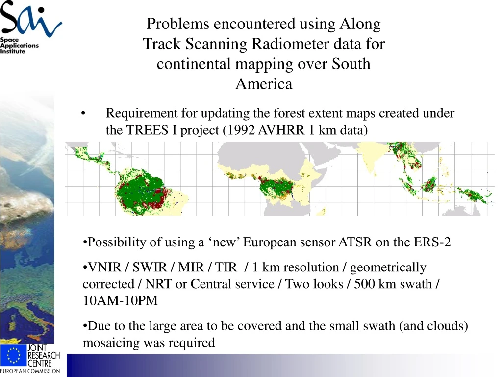
Problems encountered using Along Track Scanning Radiometer data for continental mapping over South America • Requirement for updating the forest extent maps created under the TREES I project (1992 AVHRR 1 km data) • Possibility of using a ‘new’ European sensor ATSR on the ERS-2 • VNIR / SWIR / MIR / TIR / 1 km resolution / geometrically corrected / NRT or Central service / Two looks / 500 km swath / 10AM-10PM • Due to the large area to be covered and the small swath (and clouds) mosaicing was required
Sun Satellite West of image – satellite ‘views’ illuminated canopy East of image – satellite ‘views’ into the shaded canopy
Within image spectral confusion (e.g. dense forest on west of image / degraded forest on east of image) • Biased pixel selection and spectral confusion in mosaics • Solutions? • Throw away half of each image (! We would never have enough data) • corrections based on known BRDF models of landcover (need to know the cover type) • construct the models for our database and then invert (atmospheric contamination of haze effects the data base)
In practice – used the RPV (Rahman et al. 1993) – Empirical coefficients are used along with the Sun-Target-Sensor geometry to correct the data. p corrected = p(v,u,φ,j, k, H) v,u,φ – are viewing geometry angles J,k,H are optimised coefficient
Problems • unable to adequately establish stable parameters for the RPV polynomial (atmospheric contamination?) • the available time series was too erratic – not enough images in certain areas and in certain seasons • Mosaics were produced – • Highest Tsurface (“tropical dry season”) (clean images but highly contrasted) • Highest NDVI (“tropical wet season”) (pixelated) • - Lowest SWIR (“moist / shadowed”) (cloud shadow and haze)
Highest Tsurface Lowest SWIR
Ts NDVI SWIR Mosaicing used as a means of selecting the best images for particular seasons Input images Output mosaics • smaller mosaics then constructed for ecological regions
Lessons for VGT data • the same problem exists • the exceptional data availability means that compositing should be more feasible
Need for: • BRDF corrected images – if possible independent of existing land cover classification • Mosaicing techniques that reflect vegetation in different states – “dry” and “wet” season images and avoid the following problems • Cloud shadow • Haze • Smoke • “Pixelation”