Download

1 / 45
450 likes | 680 Vues
Hidden Markov Model . 11/28/07. Bayes Rule. The posterior distribution Select k with the largest posterior distribution. Minimizes the average misclassification rate. Maximum likelihood rule is equivalent to Bayes rule with uniform prior. Decision boundary is . Naïve Bayes approximation.

E N D
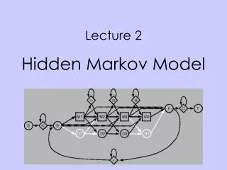
Hidden Markov Model 11/28/07
Bayes Rule The posterior distribution Select k with the largest posterior distribution. Minimizes the average misclassification rate. Maximum likelihood rule is equivalent to Bayes rule with uniform prior. Decision boundary is
Naïve Bayes approximation • When x is high dimensional, it is difficult to estimate
Naïve Bayes Classifier • When x is high dimensional, it is difficult to estimate • But if we assume independence, then it becomes a 1-D problem.
Naïve Bayes Classifier • Usually the independence assumption is not valid. • But sometimes the NBC can still be a good classifier. • A lot of times simple models may not perform badly.
A coin toss example Scenario: You are betting with your friend using a coin toss. And you see (H, T, T, H, …)
A coin toss example Scenario: You are betting with your friend using a coin toss. And you see (H, T, T, H, …) But, you friend is cheating. He occasionally switches from a fair coin to a biased coin – of course, the switch is under the table! Biased Fair
A coin toss example This is what really happening: (H, T, H, T,H, H, H, H, T,H, H, T, …) Of course you can’t see the color. So how can you tell your friend is cheating?
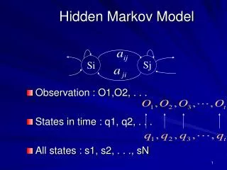
Hidden Markov Model Hidden state (the coin) Observed variable (H or T)
Markov Property Hidden state (the coin) Observed variable (H or T)
Markov Property transition probability prior distribution Biased Fair
Observation independence Hidden state (the coin) Observed variable (H or T) Emission probability
Model parameters A = (aij) (transition matrix) p(yt | xt) (emission probability) p(x1) (prior distribution)
Model inference • Infer states when model parameters are known. • Both states and model parameters are unknown.
Viterbi algorithm time t-1 t t+1 1 2 state 3 4
Viterbi algorithm time • Most probable path: t-1 t t+1 1 2 state 3 4
Viterbi algorithm time • Most probable path: t-1 t t+1 1 2 state 3 4
Viterbi algorithm time • Most probable path: t-1 t t+1 1 2 state 3 4 Therefore, the path can be found iteratively.
Viterbi algorithm time • Most probable path: t-1 t t+1 1 2 state 3 4 Let vk(i) be the most probable path ending in state k. Then
Viterbi algorithm • Initialization (i=0): • Recursion (i=1,...,L): • Termination: • Traceback (i = L, ..., 1):
Advantage of Viterbi path • Identify the most probable path very efficiently. • The most probable path is legitimate, i.e., it is realizable by the HMM process.
Issue with Viterbi path • The most probability path does not predict the confidence level of a state estimate. • The most probably path may not be much more probable then other paths.
Posterior distribution Estimate p(xk | y1, ..., yL). Strategy: This is done by a forward-backward algorithm
Forward-backward algorithm Estimate fk(i)
Forward algorithm Estimate fk(i) Initialization: Recursion: Termination:
Backward algorithm Estimate bk(i)
Backward algorithm Estimate bk(i) Initialization: Recursion: Termination:
Probability of fair coin 1 P(fair)
Probability of fair coin 1 P(fair)
Posterior distribution • Posterior distribution predicts the confidence level of a state estimate. • Posterior distribution combines information from all paths. But.. • The predicted path may not be legitimate.
Estimating parameters when state sequence is known Given the state sequence {xk} Define Ajk = # transitions from j to k. Ek(b) = #emissions of b from k. The maximum likelihood estimates of parameters are:
Infer hidden states together with model parameters • Viterbi training • Baum-Welch
Viterbi training Main idea: Use an iterative procedure • Estimate state for fixed parameters using the Viterbi algorithm. • Estimate model parameters for fixed states.
Baum-Welch algorithm • Instead of using the Viterbi path to estimate state, consider the expected number of Akl and Ek(b)
Baum-Welch algorithm • Instead of using the Viterbi path to estimate state, consider the expected number of Akl and Ek(b)
Baum-Welch is a special case of EM algorithm • Given an estimate of parameter qt , try to find a better q. • Choose q to maximize Q
Baum-Welch is a special case of EM algorithm • E-step: Calculate the Q function • M-step: Maximize Q(q|qt) with respect to q.
Issue with EM • EM only finds local maxima. • Solution: • Run multiple EM starting with different initial guesses. • Use more sophisticated algorithm such as MCMC.
Dynamic Bayesian Network Kelvin Murphy
Software • Kevin Murphy’s Bayes Net Toolbox for Matlab http://www.cs.ubc.ca/~murphyk/Software/BNT/bnt.html
Applications Copy number changes (Yi Li)
Applications Protein-binding sites
Applications Sequence alignment www.biocentral.com
Reading list • Hastie et al. (2001) the ESL book • p184-185. • Durbin et al. (1998) Biological Sequence Analysis • Chapter 3.