Download
1 / 12
120 likes | 253 Vues
March 2010 Refraction Survey Applied Geophysics – 492 John Louie. Patricia Capistrant & Troy Christensen. Introduction To Refraction.

E N D
March 2010 Refraction SurveyApplied Geophysics – 492 John Louie Patricia Capistrant & Troy Christensen
Introduction To Refraction • -Seismic refraction surveying provides earth scientists and engineers with information that is contiguous along survey lines placed in areas of interest. Refraction surveys are rapid and cost-effective, and can be conducted using as few as two to three people in the field. Certain applications actually allow target features to be recognized during the field survey such as faults or other structures at depth. Photo from Louie
Introduction To RefractionContinued Common Applications Determine depth to water table. Determine depth to bedrock. Locate fractures zones in bedrock. Bulk, shear, and Young’s Modulus, and Poisson’s ratio. Measure thickness of aggregate deposits. Determine depth to base of backfilled quarries. Determine depth of landfills. Determine thickness of overburden. Map topography of groundwater. How it works When a seismic wave reaches a layer of higher velocity a portion of the energy is refracted, or bent, and travels along the refractor as a compressional wave at a velocity determined by the composition of the refractor (bedrock). Energy from the propagating wave leaves the refractor at the “critical angle” of refraction and returns to the surface. The angle of refraction depends on the composition in the refractor and the material it is in contact with (Snell’s Law). Both compressional waves (P-waves) and shear waves (S-waves) can be used in the seismic refraction method, although compressional waves are most commonly utilized. The seismic wave can be generated from a variety of sources that include a hammer and plate, weight drop, elastic wave generator, or small seis-gun (shotgun cartridge), all of which are non-intrusive on the surface. The seismic wave energy is detected with an array of linearly spaced geophones and recorded. The recorded signals are processed to determine travel-times of the refracted energy, thus allowing the depth profile of the refractor to be constructed.
Methods • A total of 3 refraction surveys were run during the Spring Break, 2010 experiment. The first ran north-south from Windy Hill to the corner of Manzanita and Plumas. The second ran north-south from Reno’s Auto Museum to the northern end of the University of Nevada. The third refraction experiment ran east-west from the corner of Plumas and Manzanita, west to the corner of Manzanita and W. McCarren Blvd. • Everyday the Texans were utilized for a refraction experiment, they were programmed with a date using a gps unit, and were programmed to turn on and off at a given time. Likewise the data collected on the Texans then had to be downloaded and unencrypted to readable files through the use of DOS and MAC programs.
Methods Continued Before Deployment Texans programmed with day and time using a gps unit. Any unwanted data erased off the memory of the Texans. Battery voltage checked and batteries replaced if necessary. An event table created to store new data, and a time programmed to turn on and off the data acquisition systems. Deployment Planned dispersion of Texans with an equal distance of spacing between them. 5 minute cluster test before deployment recording time of start and end and gps coordinates. Deploy the individual Texans and record the time that the unit was placed in the ground, and the coordinates given by a gps specific to that unit. Mark that unit by flagging it. Wait for the generated seismic event.
Methods Continued Recording The Event 5 Texans were designated to have a seismic source applied adjacent to them. The Texans selected are spaced evenly with one at each end of the line and 3 evenly spaced in the middle. A geophone and Texan followed the seismic source throughout the line recording a gps location and time of hammer hits at each location. Collection After the seismic event, the Texans and geophones were pulled with the time recorded that each was pulled. A 5 minute cluster test was then run on all of the devices gathered. Finally the devices were taken back to the university where they were programmed to send the gathered data to the event table created. Then each Texan was reset for the next test with a day and time, and the old data erased off of the devices memory.
Results • This refraction experiment did not yield any useful results. Therefore, no conclusions could be inferred from the data that was gathered. • In the shot records that were observed, there were no apparent first arrivals that matched the event, or that were refracted from a structure. Thus the data collected from the devices was rendered useless with regards to this experiment. • In addition to these results and contributing to a lack of data, one of the three lines used in this experiment failed to collect any data.