Download
1 / 36
390 likes | 990 Vues
The Fast Fourier Transform (and DCT too…). Nimrod Peleg Oct. 2002. Outline . Introduce Fourier series and transforms Introduce Discrete Time Fourier Transforms, (DTFT) Introduce Discrete Fourier Transforms (DFT) Consider operational complexity of DFT Deduce a radix-2 FFT algorithm

E N D
The Fast Fourier Transform(and DCT too…) Nimrod Peleg Oct. 2002
Outline • Introduce Fourier series and transforms • Introduce Discrete Time Fourier Transforms, (DTFT) • Introduce Discrete Fourier Transforms (DFT) • Consider operational complexity of DFT • Deduce a radix-2 FFT algorithm • Consider some implementation issues of FFTs with DSPs • Introduce the sliding FFT (SFFT) algorithm
The Frequency Domain • The frequency domain does not carry any information that is not in the time domain. • The power in the frequency domain is that it is simply another way of looking at signal information. • Any operation or inspection done in one domain is equally applicable to the other domain, except that usually one domain makes a particular operation or inspection much easierthan in the other domain. • frequency domain information is extremely important and useful in signal processing.
3 Basic Representations for FT • 1. An Exponential Form • 2. A Combined Trigonometric Form • A Simple Trigonometric Form
Complex Numbers ! The Fourier Series: Exponential Form Periodic signal expressed as infinite sum of sinusoids. • Ck’s are frequency domain amplitude and phase representation • For the given value xp(t) (a square value), the sum of the first four terms of trigonometric Fourier series are: xp(t) 1.0 + sin(t) + C2sin(3t) + C3sin(5t)
The Combined Trigonometric Form • Periodic signal: xp(t) = xp(t+T) for all t and cycle time (period) is: f0 is the fundamental frequency in Hz w0 is the fundamental frequency in radians: xp(t) can be expressed as an infinite sum of orthogonal functions. When these functions are the cosine and sine, the sum is called the Fourier Series. The frequency of each of the sinusoidal functions in the Fourier series is an integer multiple of the fundamental frequency. Basic frequency + Harmonies
Fourier Series Coefficients • Each individual term of the series, ,is the frequency domain representation and is generally complex (frequency and phase), but the sum is real. • The second common form is the combined trigonometric form: Again: Ck are Complex Numbers !
The Trigonometric Form All three forms are identical and are related using Euler’s identity: Thus, the coefficients of the different forms are related by:
The Fourier Transform1/3 The Fourier series is only valid for periodic signals. For non-periodic signals, the Fourier transformis used. Most natural signals are not periodic (speech). We treat it as a periodic waveform with an infinite period. If we assume that TPtends towards infinity, then we can produce equations (“model”) for non-periodic signals. If Tp tends towards infinity, then w0 tends towards 0. Because of this, we can replace w0 with dw, and it leads us to:
The Fourier Transform 2/3 • Increase TP = Period Increases : No Repetition: • Discrete frequency variable becomes continuous: • Discrete coefficients Ck become continuous:
The Fourier Transform 3/3 We define:
Signal Representation by Delta Function Instead of a continuous signal we have a “collection of samples”: This is equivalent to sampling the signal with one Delta Function each time, moving it along X-axis, and summing all the results: Note that the Delta is “1” only If its index is zero !
Discrete Time Fourier Transform 1/3 • Consider a sampled version, xs(t) , of a continuous signal, x(t) : Ts is the sample period. We wish to take the Fourier transform of this sampled signal. Using the definition of Fourier transform of xs(t) and some mathematical properties of it we get: • Replace continuous time t with (nTs) • Continuous x(t) becomes discrete x(n) • Sum rather than integrate all discrete samples
Discrete Time Fourier Transform 2/3 Fourier Transform Discrete Time Fourier Transform Inverse Discrete Time Fourier Transform Inverse Fourier Transform • Limits of integration need not go beyond ± because the spectrum repeats itself outside ± (every 2): • Keep integration because is continuous: means that is periodic every Ts
Discrete Time Fourier Transform 3/3 • Now we have a transform from the time domain to the frequency domain that is discrete, but ... DTFT is not applicable to DSP because it requires an infinite number of samples and the frequency domain representation is a continuous function – impossible to represent exactly in digital hardware.
1st result: Nyquist Sampling Rate 1/2 • The Spectrum of a sampled signal is periodic, with 2*Pi Period: Easy to see:
1st result: Nyquist Sampling Rate 2/2 • For maximum frequency wH :
Practical DTFT • Take only N time domain samples • Sample the frequency domain, i.e. only evaluate x() at N discrete points. The equal spacing between points is = 2/N
The DFT Since the only variable in is k , the DTFT is written: The result is called Discrete Fourier Transform (DFT): Using the shorthand notation: (Twiddle Factor)
Usage of DFT • The DFT pair allows us to move between the time and frequency domains while using the DSP. • The time domain sequence x[n] is discrete and has spacing Ts, while the frequency domain sequence X[k] is discrete and has spacing 1/NT [Hz].
N Samples X(n) |x(k)| N Samples 0 Ts 2Ts 3Ts (N-1)Ts 0 1 2 3 N-1 t k N-2 N-1 0 1 2 N/2 n 0 f DFT Relationships Time Domain Frequency Domain
Each term such as requires 8 multiplications Practical Considerations • Standard DFT: • An example of an 8 point DFT: • Writing this out for each value of n : • Total number of (complex !) multiplications required: 8 * 8 = 64 • 1000-point DFT requres 10002 = 106 complex multiplications • And all of these need to be summed….
Fast Fourier Transform Symmetry Property Periodicity Property Splitting the DFT in two (odd and even) or Manipulating the twiddle factor THE FAST FOURIER TRANSFORM
FFT complexity (N/2)2 multiplications (N/2)2 multiplications N/2 Multiplications • For an 8-point FFT, 42 + 42 + 4 = 36 multiplications, saving 64 - 36 = 28 multiplications • For 1000 point FFT, 5002 + 5002 + 500 = 50,500 multiplications, saving 1,000,000 - 50,500 = 945,000 multiplications
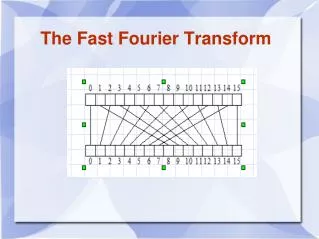
Splitting the original series into two is called decimation in time • Let us take a short series where N = 8 • Decimate once Called Radix-2 since we divided by 2 n = {0, 1, 2, 3, 4, 5, 6, 7} n = { 0, 2, 4, 6 } and { 1, 3, 5, 7 } • Decimate again n = { 0, 4 } { 2, 6 } { 1, 5 } and { 3, 7 } Time Decimation • The result is a savings ofN2 – (N/2)log2N multiplications: • 1024 point DFT = 1,048,576 multiplications • 1024 point FFT = 5120 multiplication • Decimation simplifies mathematics but there are more twiddlefactors to calculate, and a practical FFT incorporates these extra factors into the algorithm
Decimate in time into 2 series: n = {0 , 2} and {1, 3} Simple example: 4-Point FFT • Let us consider an example where N=4: • We have two twiddle factors. • Can we relate them? • Now our FFT becomes:
x(0) + + W40 x(2) W40 x(1) + W40 x(3) 4-Point FFT Flow Diagram The 2 DFT’s: for k=0,1,2,3 For k=0 only: A ‘flow-diagram’ of it: This is for only 1/4 of the whole diagram !
Note: X4(0) x(0) 0 0 X4(1) x(2) 2 1 X4(2) 2 x(1) 0 X4(3) 3 x(3) 2 A Complete Diagram
Twiddle Conversions A Typical Butterfly 0 W4 = 1 x1 + x1 k = x2 X1 WN X1 1 W4 = -j k WN 2 = -1 W4 x2 X2 x1 – k = x2 X2 WN 3 = j W4 4 Point FFT Butterfly 4 Point FFT Equations x0 X0 0 X0 = (x0 + x2) + W4 (x1+x3) 1 X1 = (x0 – x2) + W4 (x1–x3) X1 x2 0 W4 0 X2 = (x0 + x2) – W4 (x1+x3) x1 X2 1 X3 = (x0 – x2) – W4 (x1–x3) 1 W4 x3 X3 The Butterfly
Summary • Frequency domain information for a signal is important for processing • Sinusoids can be represented by phasors • Fourier series can be used to represent any periodic signal • Fourier transforms are used to transform signals • From time to frequency domain • From frequency to time domain • DFT allows transform operations on sampled signals • DFT computations can be sped up by splitting the original series into two or more series • FFT offers considerable savings in computation time • DSPs can implement FFT efficiently
Bit-Reversal • If we look at the inputs to the butterfly FFT, we can see that the inputs are not in the same order as the output. • To perform an FFT quickly, we need a method of shuffling these input data addresses around to the correct order. • This can be done either by reversing the order of the bits that make up the address of the data, or by pointer manipulation (bit reversed addition). • Many DSPs have special addressing modes that allow them to automatically shuffle the data in the background.
X4(0) x(0) 0 0 X4(1) x(2) 2 1 X4(2) 2 x(1) 0 X4(3) 3 x(3) 2 Bit-Reversal example • To obtain the output in ascending order the input values must be loaded in the order: {0,2,1,3} • for 512 or 1024 it is much more complicated...
8-point Bit-Reversal • Consider a 3-bit address (8 possible locations). • After starting at zero, we add half of the FFT length at each address access with carrying from left to right (!) Start at 0 = 000 =x(0) 000+100 = 100 =x(4) 100+100 = 010 =x(2) 010+100 = 110 =x(6) 110+100 = 001 =x(1) 001+100 = 101 =x(5) 101+100 = 011 =x(3) 011+100 = 111 =x(7) Note that reversing the order of the address bits gives same result !
And what about DCT ??? The rest of the math is quite similar….. DCT Type II*: Note: at least 4 types of DCT !!! * after: A course in Digital Signal Processing, Boaz Porat
Type I Type II Type III Type IV DCT Basis Vectors for N=8 DCT Type II Most used for compression: JPEG, MPEG etc.
DCT Features • Real transformation • Reversible transformation • 2D Transformation exists and separable • Better than the DFT as a “de-correlator” • Fast algorithm exists (NlogN Complexity)