Download
1 / 54
550 likes | 760 Vues
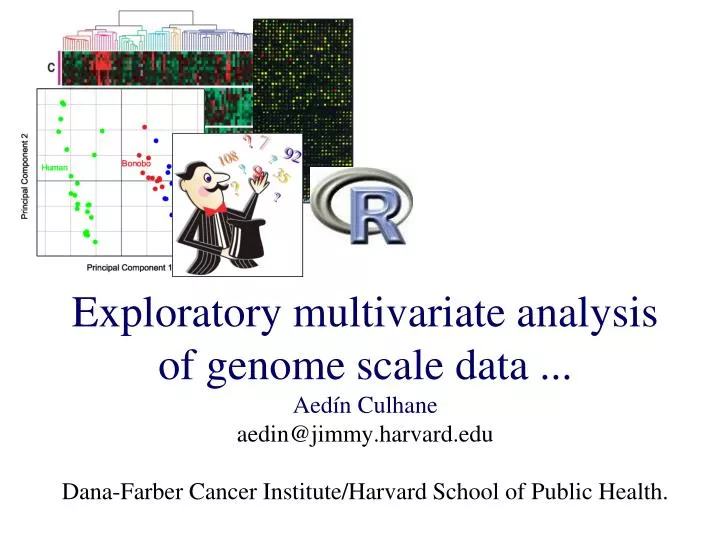
Exploratory multivariate analysis of genome scale data ... Aed ín Culhane aedin@jimmy.harvard.edu Dana-Farber Cancer Institute/Harvard School of Public Health. Why do we do exploratory data analysis?. Genome scale data 10,000’s variables Multivariate

E N D
Exploratory multivariate analysis of genome scale data ...Aedín Culhaneaedin@jimmy.harvard.eduDana-Farber Cancer Institute/Harvard School of Public Health.
Why do we do exploratory data analysis? • Genome scale data • 10,000’s variables • Multivariate • Essential to use exploratory data analysis to “get handle” on data
Exploration of Data is Critical • Detect unpredicted patterns in data • Decide what questions to ask • Can also help detect cofounding covariates
A 6 gene signature of lung metastasis Landemaine T et al., Cancer Res. 2008 Aug 1;68(15):6092-9.
But metastatic profile of breast cancer differs by tumor subtype Smid et al., 2008 Cancer Res 68(9):3108–14
Confounding Covariates Culhane AC & Quackenbush J. 2009 Cancer Research
Importance of Data Exploration • Exploration of Data is Critical • Clustering • Hierarchical • Flat (k-means) • Ordination (Dimension Reduction) • Principal Component analysis, Correspondence analysis
A Distance Metric • In exploratory data analysis • only discover where you explore.. • The choice of metric is fundamental
Distance Similarity Distance Metrics • Euclidean distance • Pearson correlation coefficient • Spearman rank • Manhattan distance • Mutual information • etc Each has different properties and can reveal different features of the data
Clustering: Distance metrics • Euclidean distance • A commonly used measure Pythagorean Theorem h2=a2+b2 h=√a2+b2 X1,Y1 h = √(X2-X1)2 +(Y2-Y1)2 a=X2-X1 b=Y2-Y1 X2,Y2
Exp 1 Exp 2 Exp 3 Exp 4 Exp 5 Exp 6 Gene A x1A x2A x3A x5A x4A x6A pB Gene B x1B x2B x3B x4B x5B x6B • Euclidean: i = 1(xiA - xiB)2 6 pA 2. Pearson correlation Distance Metrics
Distance Metric: EuclideanPearson* 1.4 -0.05 D D 6.0 +1.00 Distance Is Defined by a Metric
Correlations gone wrong Random Noise rnorm(10, mean=1, sd=2) y=x/2+1
dist() hclust() heatmap() library(heatplus) Cluster Analysis
Relationships between these pairwise distances- Clustering Algorithms • Different algorithms • Agglomerative or divisive • Popular hierarchical agglomerative clustering method • The distance between a cluster and the remaining clusters can be measured using minimum, maximum or average distance. • Single lineage algorithm uses the minimum distance.
Comparison of Linkage Methods Average Single Complete Join by min average max
A B Quick Aside: Interpreting hierarchical clustering trees Hierarchical analysis results viewed using a dendrogram (tree) • Distance between nodes (Scale) • Ordering of nodes not important (like baby mobile) Tree A and B are equivalent
Limitations of hierarchical clustering • Samples compared in a pair wise manner • Hierarchy forced on data • Sometimes difficult to visualise if large data • Overlapping clustering or time/dose gradients ?
Complementary methods Cluster analysis generally investigates pairwise distances/similarities among objects looking for fine relationships Ordination in reduced space considers the variance of the whole dataset thus highlighting general gradients/patterns (Legendre and Legendre, 1998)
Ordination • Also refers to as • Latent variable analysis, Dimension reduction • Aim:Find axes onto which data can be project so as to explain as much of the variance in the data as possible
z New Axis 1 New Axis 2 New Axis 3 y x Dimension Reduction (Ordination) Principal Componentspick out the directionsin the data that capturethe greatest variability
Representing data in a reduced space New Axis 2 New Axis 1 The first new axes will be projected through the data so as to explain the greatest proportion of the variance in the data. The second new axis will be orthogonal, and will explain the next largest amount of variance
Interpreting an Ordination Each axes represent a different “trend” or set of profiles The further from the origin Greater loading/contribution (ie higher expression) Same direction from the origin
Principal Axes • Project new axes through data which capture variance. Each represents a different trend in the data. • Orthogonal (decorrelated) • Typically ranked: First axes most important • Principal axis, Principal component, latent variable or eigenvector
Typical Analysis Plot of eigenvalues, select number. X Ordination Array Projection Gene Projection Plot PC1 v PC2 etc
Eigenvalues • Describe the amount of variance (information) in eigenvectors • Ranked. First eigenvalue is the largest. • Generally only examine 1st few components • scree plot
Choosing number of Eigenvalues: Scree Plot Maximum number of Eigenvalues/Eigenvectors = min(nrow, ncol) -1
Ordination Methods Most common : • Principal component analysis (PCA) • Correspondence analysis (COA or CA) • Principal co-ordinate analysis (PCoA, classical MDS) • Nonmetric multidimensional scaling (NMDS, MDS) Interpreting a
Relationship • PCA, COA, etc can be computed using Singular value decomposition (SVD) • SVD applied to microarray data (Alter et al., 2000) • Wall et al., 2003 described both SVD, PCA (good paper)
Summary: Exploration analysis using Ordination • SVD = straightforward dimension reduction • PCA = column mean centred +SVD • Euclidean distance • COA = Chi-square +SVD • produces nice biplot • Ordination be useful for visualising trends in data • Useful complementary methods to clustering
Ordination (PCA, COA) library(ade4) dudi.pca() dudi.coa() library(made4) ord(data, type=“pca”) plot() plotarrays() plotgenes() Ordination in R Link to example 3d html file
An Example and Comparison • Karaman, Genome Res. 2003 13(7):1619-30. • Compared fibroblast gene signature from 3 species
Coding Region : Introns, Exons and Internal Repeats MAR, Alu, CpG, Promoter Poly A, MAR Integrate Data Sets?
Data Production Line • DNA • SNP • Array CGH • RNA • Microarray • microRNA, Tiling arrays • Proteins • Mass Spec, LC-MS etc • 2D gels • Protein Interaction • Metabolites
Multivariate Methods to detecting co-related trends in data • Canonical correlation analysis • Partial least squares • Co-inertia analysis
Coinertia Analysis • Useful for cross-platform comparison where the same samples have been arrayed. • Identifies correlated “trends” in data • Consensus and divergence between gene expression profiles from different DNA microarray platforms are graphically visualised. • Not dependent on annotation thus can extract important genes even when there are NOT present across all datasets. Culhane, A.C., Perriere, G., Higgins D.G., (2003) Cross platform comparison and visualisation of gene expression data using co-inertia analysis. BMC Bioinformatics, 4:59
colon cell line HT29 • spotted • - Affymetrix CIA of NCI60 cell line datasets
Melanoma markers on Affymetrix not on Stanford array Projection of Affymetrix genes Ordinations of arrays of cell lines
G1 -- -- -- -- -- -- -- -- -- -- -- -- -- -- -- -- -- -- -- -- -- -- -- Gr P1 -- -- -- -- -- -- -- -- -- -- -- -- -- Pq Coupling Genes, Proteins + GO Terms Gene Expression Data Proteomics Data Use CIA to find correlated trends in genomics & proteomics data. Project GO terms on these axes to aid in interpretation of results S1 - - - - - - Sn S1 - - - - - - Sn
Gene expression and proteomics data from the life cycle of the malarial parasitic. Sample with variables (tri-plot) RV coefficient = 0.88.
Project GO terms on Genes & Proteins space. Variables Sample with variables (tri-plot) GO Terms Axis 1 (horizontal) Accounts for 24.6% variance. Splits sexual & asexual life stages Axis 2 (vertical) 4.8% variance. Splits invasive stages (Merozoite and Sporozoite stages which invade red blood)
Detecting translationally repressed genes Known: translationally repressed in female Gametocyte stage of Plasmodium berghei. These genes silence in the gametocyte stage but once ingested by mosquito, undergo translation into their respective proteins.Examined Plasmodium falciparum orthologs CIA: See genes transcriptionally active but their protein product is absent in the gametocyte stage.
Visualising Genes, Proteins and GO terms • CIA useful particularly to visualize variant “opposing” trends • Addition of GO terms may assist when lack protein annotation (MS/MS data) • Can be extended to supplement any annotation terms. Fagan A, Culhane AC, Higgins DG. (2007) A Multivariate Analysis approach to the Integration of Proteomic and Gene Expression Data. Proteomics.7(13):2162-71.
G1 -- -- -- -- -- -- -- -- -- -- -- -- -- Gn G1 -- -- -- -- -- -- -- -- -- -- -- -- -- Gn Using Semi-Supervised CIA to detect association between Gene Expression and Motifs Frequency of TFBS TFBS1 - - - - - TFBSn Gene Expression Data Class1 Class2 Class3