Download

1 / 35
350 likes | 536 Vues
Asset Pricing in the Presence of Background Risk. Andrei Semenov (York University). Introduction. The standard consumption CAPM: Problems: a) The equity premium puzzle b) The risk-free rate puzzle. Generalizations: a) Preference modifications b) State-dependent parameters

E N D
Asset Pricing in the Presence of Background Risk Andrei Semenov (York University)
Introduction The standard consumption CAPM: Problems: a) The equity premium puzzle b) The risk-free rate puzzle
Generalizations: a) Preference modifications b) State-dependent parameters c) Psychological models of preferences d) Incomplete consumption insurance Brav et al. (2002), Balduzzi and Yao (2007), and Kocherlakota and Pistaferri (2009)
Outline • Consumption-Based Model with Background Risk • The stochastic discount factor (SDF) • Risk vulnerability and the asset pricing puzzles • Risk aversion and the EIS under background risk • Empirical Investigation • The data • The estimation procedure (calibration, conditional HJ volatility bounds) • Estimation results • Concluding Remarks
1. A Consumption-based asset pricing model with background risk 1.1 The Stochastic Discount Factor (SDF) The agent faces (Franke et al. (1998) and Poon and Stapleton (2005)): • The financial investment risk • An independent, non-hedgeable, zero-mean background risk (loss of employment, divorce, etc.)
In the presence of background risk, the representative agent maximizes: is the agent i’s hedgeable consumption in period . The non-hedgeable consumption is independent of both optimal hedgeable consumption and the risky payoff and has a zero expected value.
One of the first-order conditions: or This is the consumption CAPM with background risk. The SDF: In the absence of background risk,
1.2 The precautionary premium Following Kimball (1990): where is an equivalent precautionary premium. Assume , then
We can write the SDF as: Assume that the utility function is CRRA: The precautionary premium for the agent with CRRA utility is hence
This implies that, with CRRA utility, for any t Where is the normalized variance of : We need for marginal utility to be well-defined. The SDF is then
1.3 Risk vulnerability and the asset pricing puzzles As introduced by Kihlstrom et al. (1981) and Nachman (1982), define the following indirect utility function: Gollier (2001) argues that, in the case of the background risk with a non-positive mean preferences exhibit risk vulnerability if and only if the indirect utility function is more concave than the original utility function, i.e.,
As shown by Gollier (2001), this inequality holds if at least one of the following two conditions is satisfied: (i) ARA is decreasing and convex and (ii) both ARA and AP are positive and decreasing in wealth (standard risk aversion (Kimball (1993)).
Risk vulnerability and the equity premium puzzle The consumption CAPM with background risk in terms of : Assume Then If , then is less concave than utility and hence .
1.4 Risk aversion and the EIS under background risk Suppose that at time t the agent faces the background risk and a lottery with an uncertain payoff . For any distribution functions and : The RRA coefficient
Since is independent of , and then we may suppose Denote as the risk premium we would observe if the utility curvature parameter were . The proportion of the risk premium due to the background risk in the total risk premium is
Kimball (1992) defines the temperance premium by the following condition: By analogy with the risk premium, The conditions and (the necessary conditions for risk vulnerability) imply that .
We have With power utility
The EIS in the model with an independent non-hedgeable background risk Since the representative agent with utility facing background risk has the same optimal consumption plan as the representative agent with utility in the no background risk environment, we can suppose that where and The model with background risk enables us to disentangle the curvature parameter and the EIS in the expected utility framework.
2. Empirical investigation 2.1 The data • The consumption data Quarterly consumption data (consumption of nondurables and services (NDS)) from the CEX (the US Bureau of Labor Statistics) from 1982:Q1 to 2003:Q4. We drop households a) that do not report or report a zero value of consumption of food, consumption of nondurables and services, or total consumption,
b) nonurban households, households residing in student housing, households with incomplete income responses, households that do not have a fifth interview, and households whose head is under 19 or over 75 years of age. We consider four sets of households based on the reported amount of asset holdings at the beginning of a 12-month recall period in constant 2005 dollars: a) all households, b) households with total asset holdings > $ 0, c) households with total asset holdings $ 1000, d) households with total asset holdings $ 5000.
The returns data a) The nominal quarterly value-weighted market capitalization-based decile index returns (capital gain plus all dividends) on all stocks listed on the NYSE, AMEX, and Nasdaq are from the CRSP. b) The nominal quarterly value-weighted returns on the five and ten NYSE, AMEX, and Nasdaq industry portfolios are from Kenneth R. French's web page. c) The nominal quarterly risk-free rate is the 3-month US Treasury Bill secondary market rate from the Federal Reserve Bank of St. Louis. d) The real quarterly returns are calculated as the quarterly nominal returns divided by the 3-month inflation rate based on the deflator defined for NDS.
2.2 The empirical SDF Under Background risk: Recall that In any state s, . Since the background risk has a zero-mean,
2.3 The estimation We candidate SDFs are 1. Standard SDF: 2. The SDF in Brav et al. (2002): 3. The SDF in the consumption CAPM with background risk:
For each of the above SDFs, we test the conditional Euler equations for the excess returns on risky assets and the risk-free rate Denote the error terms in the Euler equations as Thus, at the true parameter vector, where is a variable in the agent's time t information set.
Calibration and HJ volatility bounds We calculate the statistic Denote as the utility curvature parameter in . The optimal value of the estimate of the curvature parameter is Denote as the instrument , for which
Since or equivalently we estimate the subjective time discount factor as and the RRA coefficient as
A lower volatility bound for admissible SDFs , which have unconditional mean m and satisfy where is the unconditional variance-covariance matrix of . We look for the values of the SDF parameters, at which a considered SDF satisfies the volatility bound, i.e., where
Concluding remarks • Empirical evidence is that, in contrast with the previously proposed incomplete consumption insurance models, the asset-pricing model with the SDF calculated as the discounted ratio of expectations of marginal utilities over the non-hedgeable consumption states at two consecutive dates jointly explains the cross-section of risky asset excess returns and the risk-free rate with economically plausible values of the RRA coefficient and the subjective time discount factor. • The results are robust across different sets of stock returns and threshold values in the definition of asset holders.
The size of the background risk is an important component of the pricing kernel. This supports the hypothesis that the independent non-hedgeable zero-mean background risk can account for the market premium and the return on the risk-free asset.