Download
1 / 22
350 likes | 757 Vues
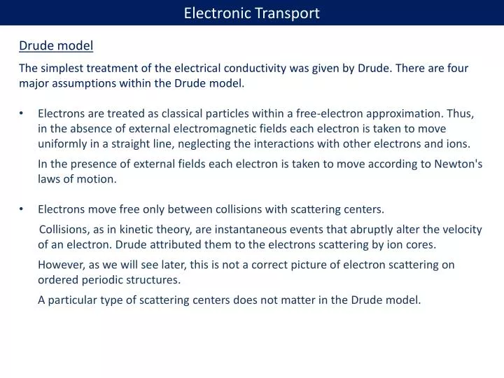
Electronic Transport. Drude model The simplest treatment of the electrical conductivity was given by Drude . There are four major assumptions within the Drude model .

E N D
Electronic Transport • Drudemodel • The simplest treatment of the electrical conductivity was given by Drude. There are four major assumptions within the Drude model. • Electrons are treated as classical particles within a free-electron approximation. Thus, in the absence of external electromagnetic fields each electron is taken to move uniformly in a straight line, neglecting the interactions with other electrons and ions. • In the presence of external fields each electron is taken to move according to Newton's laws of motion. • Electrons move free only between collisions with scattering centers. • Collisions, as in kinetic theory, are instantaneous events that abruptly alter the velocity of an electron. Drudeattributed them to the electrons scattering by ion cores. • However, as we will see later, this is not a correct picture of electron scattering on ordered periodic structures. • A particular type of scattering centers does not matter in the Drude model.
An electron experiences a collision, resulting in an abrupt change in its velocity, with a probability per unit time 1/τ. This implies that the probability of an electron undergoing a collision in any infinitesimal time interval of length dtis just dt/ τ. The time τis therefore an average time between the two consecutive scattering events. It known as the collision time (relaxation time). • It follows from this assumption that an electron picked at random at a given moment will, on the average, travel for a time τbefore its next collision. The relaxation time τis taken to be independent of an electron's position and velocity. • Electrons are assumed to achieve thermal equilibrium with their surroundings only through collisions. These collisions are assumed to maintain local thermodynamic equilibrium in a particularly simple way: immediately after each collision an electron is taken to emerge with a velocity that is not related to its velocity just before the collision, but randomly directed.
Electrical conductivity of a metal We define the conductivity which is the proportionality constant between the current density j and the electric field E at a point in the metal: j = σE The current density j is a vector, parallel to the flow of charge, whose magnitude is the amount of charge per unit time crossing a unit area perpendicular to the flow. Thus if a uniform current I flows through a wire of length L and cross-sectional area A, the current density will be j = I/A. Since the potential drop along the wire will be V = EL, we get I/A=σV/L, and hence R = L/σ A =ρL/A . Here we introduced resistivity ρ =1/σ. Unlike R, σand ρ, is a property of the material, since it does not depend on the shape and size.
Now we want to express the conductivity is terms of the microscopic properties using the Drude model. If n electrons per unit volume all move with velocity v, then the current density they give rise to will be parallel to v. Furthermore, in a time dtthe electrons will advance by a distance vdt in the direction of v, so that n(vdt)A electrons will cross an area A perpendicular to the direction of flow. Since each electron carries a charge -e, the charge crossing A in the time dtwill be -nevAdt, and hence the current density isj = -nev. At any point in a metal, electrons are always moving in a variety of directions with a variety of thermal energies. The net current density is thus depends the average electronic velocity or drift velocity v. In the absence of an electric field, electrons are as likely to be moving in any one direction as in any other, v averages to zero, and, as expected, there is no net electric current density. In the presence of a field E, however, there will be a drift velocity directed opposite to the field (the electronic charge being negative). Let us find this velocity.
Consider a typical electron at time zero. Let t be the time elapsed since its last collision. Then, at time t The typical t is the mean free path τ, while average component of initial velocity is 0. Therefore, typical directed velocity is Therefore, We see that the conductivity is proportional to the density of electrons, which is not surprising since the higher the number of carriers, the more the current density. The conductivity is inversely proportional to the mass because the mass determine the acceleration of an electron in electric field. The proportionality to τ follows because τis the time between two consecutive collisions. Therefore, the larger τis, the more time for electron to be accelerated between the collisions and consequently the larger the drift velocity.
The values of relaxation time can be obtained from the measured values of electrical conductivity. For example at room temperature the resistivity of many metals lies in the range of 1-10 mΩcm. The corresponding relaxation time is of the order of 10-14 s. We treated electrons on a classical basis. How are the results modified when the quantum statistics is taken into account? Equilibrium: Various electrons are all moving - some at very high speeds - and they carry individual currents. But the total current of the system is zero, because, for every electron at velocity v there exists another electron with velocity -v, and the sum of their two currents is zero. Thus the total current vanishes due to pair wise cancellation of the electron currents. The situation changes when a field is applied. If the field is in the positive x-direction, each electron acquires a drift velocity. Thus the whole Fermi sphere is displaced to the left. As a result, some electrons - in the shaded crescent in the figure - remain uncompensated. It is these electrons which produce the observed current.
The very small displacement is due to a relatively small drift velocity. If we assume that the electric field is 0.1 V/cm, we obtain the drift velocity of 1cm/s, which is by 8 orders in magnitude smaller the Fermi velocity of electrons. The fraction of electrons which remain uncompensated is approximately v/vF. The concentration of these electrons is therefore n(v/vF),and since each electron has a velocity of approximately vF, the current density is given by j = - en(v/vF)vF = - env This is the same expression we obtained before. Therefore, formally the conductivity is expressed by the same (Drude) formula. However, physical picture is different – we observe that only the electrons at the Fermi surface are important. Since only electrons at the Fermi surface contribute to the conductance, we can define the mean free path of electrons as l=vFτ. We can make an estimate of the mean free path for metal at room temperature. This estimate gives a value of 100Å. So it is of the order of a few tens interatomic distances. At low temperatures for very pure metals the mean free path can be made as high as a few cm.
The origin of collision time We see that between two collisions, the electron travels a distance of more than 20 times the interatomic distance. This is much larger than one would expect if the electron really did collide with the ions whenever it passed them. This paradox can be explained only using quantum concepts according to which an electron has a wave character. It is well known from the theory of wave propagation in periodic structures that, when a wave passes through a periodic lattice, it continues propagating indefinitely without scattering. Therefore , if the ions form a perfect lattice, the mean free path tends to infinity, which in turn leads to infinite conductivity. It has been shown, however, that the observed l is finite (about 100 Å ). The finiteness of conductivity must thus be due to the deviation of the lattice from perfect periodicity; this happens either because of thermal vibration of the ions, or because of (2) the presence of imperfections or foreign impurities.
Normalized resistivity versus temperature for sodium, ρ (290o K) ~ 2μΩcm Residual resistance Discussion: depends on T Since 1/τ is the scattering probability we can assume that different mechanisms provide additive contributions:
At very low T, scattering by phonons is negligible because the amplitudes of oscillation are very small; in that region resistivity is almost independent of temperature. As T increases, scattering by phonons becomes more effective, and resistivity increases. When T becomes sufficiently large, scattering by phonons dominates. The statement that resistivity can be split into two part, is known as the Matthiessen rule. In general, the Matthiessen rule predicts that if there are two distinguishable sources of scattering (like in the case above – phonons and impurities) the resistivity is the sum of the resistivities due to the first and the second mechanism of scattering. The Mathissen rule is sort of empirical observation which can be used for a qualitative understanding of the contribution from different scattering mechanisms. However, one must always bear in mind the possibility a failure of this rule. In particular, in the case when the relaxation time depends on the wave vector k, the Matthissen rule becomes invalid.
Crude estimates of relaxation times Impurity scattering: Result: Phonon scattering: high temperatures atomic vibrations In the low-temperature range the lattice resistivity varies with temperature in a different way. Using the Debye model at low temperature range one can find that
Thermal conductivity When the ends of a metallic wire are at different temperatures, heat flows from the hot to the cold end. The basic experimental fact is that the heat current density, jQ, i.e. the amount of thermal energy crossing a unit area per unit time is proportional to the temperature gradient, where K is the thermal conductivity. In insulators, heat is carried entirely by phonons, but in metals heat may be transported by both electrons and phonons. The thermal conductivity K is therefore equal to the sum of the two contributions, interplay being dependent on temperature. The physical basis for thermal conductivity: Energetic electrons on the left carry net energy to the right.
Electrons at the hot end (to the left) travel in all directions, but a certain fraction travel to the right and carry energy to the cold end. Similarly, a certain fraction of the electrons at the cold end (on the right) travel to the left, and carry energy to the hot end. Since on the average electrons at the hot end are more energetic than those on the right, a net energy is transported to the right, resulting in a current of heat. Note that heat is transported entirely by electrons having the Fermi energy, because those well below this energy cancel each other's contributions. To evaluate the thermal conductivity K quantitatively, we use the formula K = (1/3) CelvFle, whereCelis the electronic specific heat per unit volume, vF is the Fermi velocity of electrons, leis the mean free path of electrons at the Fermi energy. Using expression for the heat capacity derived earlier, we find This is called the Wiedemann-Franz law. The constant of proportionality L =2.45×10⁻⁸ WΩ/K2, which is called the Lorentz number, is independent of the particular metal. It depends only on the universal constants kBand e, should be the same for all metals.
Motion in a magnetic field: cyclotron resonance and Hall effect The application of a magnetic field to a metal gives rise to several interesting phenomena due to conduction electrons. The cyclotron resonance and the Hall effect are two which we consider. Cyclotron resonance If a magnetic field is applied to a metal the Lorentz force acts on each electron. For a perfect metal in the absence of electric field the equation of motion takes the form (in CGS units ωc=eB/mc where c is the velocity of light). For magnetic fields of the order of a few kG the cyclotron frequencies lie in the range of a few GHz. The magnetic field causes electrons to move in a counter-clockwise circular fashion with the cyclotron frequency in a plane normal to the field.
Suppose now that an electromagnetic signal is passed through the slab in a direction parallel to B. The electric field of the signal acts on the electrons, and some of the energy in the signal is absorbed. The rate of absorption is greatest when the frequency of the signal is exactly equal to the frequency of the cyclotron This is so because, when ω is close to ωc (cyclotron resonance), each electron moves synchronously with the wave throughout the cycle, and therefore the absorption continues all through the cycle. Far from the resonance the electron is in phase with the wave through only a part of the cycle, during which time it absorbs energy from the wave. In the remainder of the cycle, the electron is out of phase and returns energy to the wave. Cyclotron resonance is commonly used to measure the electron mass in metals and semiconductors.
The Hall effect Let us derive an equation of motion of an electron in applied magnetic and electric field in the presence of scattering. Assume that that the momentum of an electron is p(t) at time t, let us calculate the momentum per electron p(t + dt) an infinitesimal time dt later. An electron taken at random at time t will have a collision before time t + dt, with probabilitydt/τ, and will therefore survive to time t + dtwithout suffering a collision with probability (1- dt/τ). If it experiences no collision, however, it simply evolves under the influence of the force F(due to the spatially uniform electric and/or magnetic fields) and will therefore acquire an additional momentum Fdt. The contribution of all those electrons that do not collide between tandt + dtto the momentum per electron at time t + dtis the fraction (1 - dt/τ)they constitute of all electrons, times their average momentum per electron, p(t) + Fdt. Thus neglecting for the moment the contribution to p(t + dt) from those electrons that do undergo a collision in the time between t andt + dt, we have
The correction due to those electrons that have had a collision in the interval t to t +dtis only of the order of (dt)2. To see this, first note that such electrons constitute a fraction dt/τ of the total number of electrons. Furthermore, since the electronic velocity (and momentum) is randomly directed immediately after a collision, each such electron will contribute to the average momentum p(t + dt)only to the extent that it has acquired momentum from the force F since its last collision. Such momentum is acquired over a time no longer than dt, and is therefore of order Fdt. Thus the correction order (dt/τ)Fdt, and does not affect the terms of linear order in dt. z Then the effect of individual electron collisions is to introduce a frictional damping term into the equation of motion for the momentum per electron. We apply this equation to discuss the Hall effect in metals using a free electron model. x y
Equation of motion: Stationary case: Multiply by Setting jy = 0 yields: Hall constant This is a very striking result, which predicts that the Hall coefficient depends on no parameters of the metal except the density of carriers. Since RHis inversely proportional to the electron concentration n, it follows that we can determine n by measuring the Hall field.
Some Hall coefficients are listed in a table. Note the occurrence of cases in which RH is actually positive, apparently corresponding to carriers with a positive charge. It is found experimentally that the experimental values for sodium and potassium are in excellent agreement with values calculated for one conduction electron per atom. However, for some metals the experimental values strongly disagree with the predictions of the free electron model. For example, for aluminum experiment shows that there is one positive carrier per atom, rather then three negative, as we would expect assuming the free electron model and taking into account three valence electrons. This disagreement can be explained using a band theory of solids.
Conductivity tensor: Conductivity in magnetic field is described by a tensor, it is not a scalar any more: Its reverse is the resistivity tensor:
Quantum Hall effect The Hall and diagonal magnetoresistance of an n-type GaAs-AlGaAsheterojunction for a source-drain current of 25 μA at 1.2 K.