Download

1 / 21
220 likes | 402 Vues
Unit 14. Synthesizing a Time History to Satisfy a Power Spectral Density using Random Vibration. Synthesis Purposes. A time history can be synthesized to satisfy a PSD A PSD does not have a unique time history because the PSD discards phase angle

E N D
Unit 14 Synthesizing a Time History to Satisfy a Power Spectral Density using Random Vibration
Synthesis Purposes • A time history can be synthesized to satisfy a PSD • A PSD does not have a unique time history because the PSD discards phase angle • Vibration control computers do this for the purpose of shaker table tests • The synthesized time history can also be used for a modal transient analysis in a finite element model • This is useful for stress and fatigue calculations
Random Vibration Test The Control Computer synthesizes a time history to satisfy a PSD specification.
NAVMAT P-9492 PSD Overall Level = 6.06 GRMS Accel (G^2/Hz) Frequency (Hz)
Time History Synthesis • vibrationdata > Power Spectral Density > Time History Synthesis from White Noise • Input file: navmat_spec.psd • Duration = 60 sec • Row 8, df = 2.13 Hz, dof = 256 • Save Acceleration time history as: input_th • Save Acceleration PSD as: input_psd
Base Input Matlab array: input_th
Base Input Matlab array: input_psd
SDOF System Subject to Base Excitation NESC Academy The natural frequency is Example: fn = 200 Hz, Q=10
Acceleration Response (G) max= 52.69 min= -52.56 RMS= 11.24 crest factor= 4.69 Relative Displacement (in) max= 0.01279 min=-0.01282 RMS=0.002735 The theoretical crest factor from the Rayleigh distribution = 4.58 Matlab array: response_th
Response fn=200, Q=10 The response is narrowband random. There are approximately 50 positive peaks over the 0.25 second duration, corresponding to 200 Hz.
PSD SDOF Response fn=200 Hz Q=10 Rayleigh Distribution
Response fn=200, Q=10 Matlab array: response_psd Row 8, df = 2.13 Hz, dof = 254 Peak is ~ 100 x Input at 200 Hz. Q^2 =100. Only works for SDOF system response.
Half Power Bandwidth & Curve-fit Q = fn / Δf fn = natural frequency Δf = frequency bandwidth for -3 dB points Q = 200 Hz / 20 Hz = 10 Now perform a curve-fit using the parameters shown on the next slide.