Download
1 / 48
500 likes | 521 Vues
De Novo Genome Assembly - Introduction. Henrik Lantz - NBIS/ SciLife /Uppsala University. De Novo Assembly - Scope. De novo genome assembly - not reference based Bioinformatics course - not biological interpretation Practical experience - focus on computer exercises

E N D
De Novo Genome Assembly - Introduction Henrik Lantz - NBIS/SciLife/Uppsala University
De Novo Assembly - Scope • De novo genome assembly - not reference based • Bioinformatics course - not biological interpretation • Practical experience - focus on computer exercises • Examples of programs - not exhaustive
Schedule - de novo assembly course • Monday November 14 • 09.00-09.15 Introduction (Henrik Lantz) • 09.15-10.00 Lecture: NGS technologies and basic concepts (Henrik Lantz) • 10.00-10.15 Coffee break • 10.15-10.45 Lecture: Quality control and read trimming (Mahesh Panchal) • 10.45-12.00 Exercise: Quality control and read trimming • 12.00-13.00 Lunch • 13.00-13.45 Lecture: Kmer-analysis, contamination analysis, and mapping-based analysis (Mahesh Panchal) • 13.45-15.00 Exercise: Kmer-analysis, contamination analysis, and mapping-based analysis • 15.00-15.15 Coffee break • 15.15-16.30 Team based exercise on quality control All lectures and exercises in this room!
Schedule - de novo assembly course • Tuesday November 15 • 09.00-09.30 Discussion of last day’s exercises (Henrik Lantz, Mahesh Panchal, Martin Norling) • 09.30-10.00 Lecture: Assembly basics - Genome properties (Henrik Lantz) • 10.00-10.15 Coffee break • 10.15-11.00 Lecture: Illumina assembly (Martin Norling) • 11.00-12.00 Exercise: Illumina assembly • 12.00-13.00 Lunch • 13.00-13.30 Exercise: Illumina assembly contd. • 13.30-14.30 Lecture: PacBio assembly, assembly polising, and demonstration of SMRT-portal (Mahesh Panchal) • 14.30-17.00 Exercise: PacBio assembly (incl. coffee break)
Schedule - de novo assembly course • Wednesday November 16 • 09.00-09.30 Discussion of last day’s exercises (Mahesh Panchal, Martin Norling) • 09.30-10.00 Lecture: Assembly assessment (Martin Norling) • 10.00-10.15 Coffee break • 10.15-11.00 Exercise: Assembly assessment • 11.00-11.30 Lecture: Assembly validation (Martin Norling) • 11.30-12.00 Exercise: Assembly validation • 12.00-13.00 Lunch • 13.00-13.30 Lecture: Contamination assessment (Martin Norling) • 13.30-15.00 Exercise: Assembly validation contd. + contamination assessment • 15.00-15.15 Coffee break • 15.15-15.30 Exercise discussion (Martin Norling) • 15.30-17.00 Wrap-up and project discussion
Practical info • Coffee breaks • Lunch • Dinner at Meza Grill & Bar, Östra Ågatan 11
De Novo Genome Assembly - Assembly basics Henrik Lantz - BILS/SciLife/Uppsala University
De novo genome project workflow • Extract DNA (and RNA) • Choose best sequence technology for the project • Sequencing • Quality assessment and other pre-assembly investigations • Assembly • Assembly validation • Assembly comparisons • Repeat masking? • Annotation
De novo genome project workflow • Extract DNA (and RNA)
De novo genome project workflow • Extract DNA (and RNA) • Extract much more DNA than you think you need • Also remember to extract RNA for the annotation • Single individual and haploid tissue if possible • In particular for Illumina mate-pairs data and PacBio, a lot of high molecular weight DNA is critical! • Extracting DNA for de novo assembly is very different from extractions intended for PCR • Do several extractions if possible, and run them on a gel to get an idea of how fragmented the DNA is • Try to remove contaminants from the extractions
Causes of DNA degradation Experimental setup Sample prep By Olga Vinnere Pettersson Uppsala Genome Center, SciLifeLab Mechanical damage during tissue homogenization. Wrong pH and ionic strength of extraction buffer. Incomplete removal / contamination with nucleases. Phenol: too old, or inappropriately buffered (pH 7.8 – 8.0); incomplete removal. Wrong pH of DNA solvent (acidic water). Recommended: 1:10 TE for short-term storage, or 1xTE for long-term storage. Vigorous pipetting (wide-bore pipet tips). Vortexing of DNA in high concentrations. Too many freeze-thaw cycles (we tested 5, still Ok). Debatable: sequence-dependent
What are the main contaminants? Polysaccharides Lypopolysaccharides Growth media residuals Chitin Protein Secondary metabolites Pigments Growth media residuals Chitin Fats Proteins Pigments Polyphenols Polysaccharides Secondary metabolites Pigments By Olga Vinnere Pettersson, Uppsala Genome Center, SciLifeLab
What do absorption ratios tell us? Pure DNA 260/280: 1.8 – 2.0 < 1.8: Too little DNA compared to other components of the solution; presence of organic contaminants: proteins and phenol; glycogen - absorb at 280 nm. > 2.0: High share of RNA. Pure DNA 260/230: 2.0 – 2.2 <2.0: Salt contamination, humic acids, peptides, aromatic compounds, polyphenols, urea, guanidine, thiocyanates (latter three are common kit components) – absorb at 230 nm. >2.2: High share of RNA, very high share of phenol, high turbidity, dirty instrument, wrong blank. Photometrically active contaminants: phenol, polyphenols, EDTA, thiocyanate, protein, RNA, nucleotides (fragments below 5 bp) By Olga Vinnere Pettersson, Uppsala Genome Center, SciLifeLab
DNA quality requirements Experimental setup Sample prep By Olga Vinnere Pettersson Uppsala Genome Center, SciLifeLab Some DNA left in the well Sharp band of 20+kb No sign of proteins No smear of degraded DNA No sign of RNA NanoDrop: 260/280 = 1.8 – 2.0 260/230 = 2.0 – 2.2 Qubit or Picogreen: 10 kb insert libraries: 3-5 ug 20 kb insert libraries: 10-20 ug
Experimental setup Sample prep By Olga Vinnere Pettersson Uppsala Genome Center, SciLifeLab Example:
Some general concepts • Assembly process • Coverage • Paired end/mate pair • Insert size • File formats • Contigs/scaffolds • N50
Next Generation Sequencing • Genomic DNA is fragmented (not Nanopore) and sequenced -> millions of small sequences (reads) from random parts of the genome • Depending on sequence technology, reads can be from 100 bp up to 100kb in length
De novo assembly process Genomic DNA Fragmentation + Sequencing Sequence reads Assembly Connection between reads found Consensus sequence Modified from “De Novo Genome asssembly” PDF by Torsten Seeman, Melbourne University.
Assembly Reads 5x Per base coverage 2x Assembly Overlapping reads Consensus sequence = genome Usually the haploid genome that is reported Per base coverage = number of reads that support a certain position Depth of coverage = average coverage (often shortened to “coverage” or “depth”)
Depth of coverage • Coverage = (number of reads x read length)/genome size • Example 1: (10e+6 reads x 100 bps)/10e+6= 100x coverage
Depth of coverage • Example 2: I know that the genome I am sequencing is 10 Mbases. I want a 50x coverage to do a good assembly. I am ordering 125 bp Illumina reads. How many reads do I need? • (125xN)/10e+6=50 • N=(50x10e+6)/125=4e+6 (4 million reads) • A Illumina lane gives you 180x2 million reads (PE)
Insert size Insert size Read 1 DNA-fragment Read 2 Adapter+primer Inner mate distance
Mate-pair Used to get long Insert-sizes
Orientation of paired reads Paired end (PE) reads Mate pair (MP) reads
Fastq format @D00118:257:C8672ANXX:2:2302:2055:2109 1:N:0:GAGATTCC+GTACTGAC CGTAGCCCTGTGCGACGGTGTCCGACTGCACGTCGCCGTCGTAGTTCTTGCACGCCCAGACGTAACCGCCTTCCC + 3:>@BGGGGGGGGGGGGGGGGGGGGGGGGGGGGGGGGGGGGGGGGGECGGFGGGGGGGGGGGGGGGGGG The names follow this format: @<instrument>:<run number>:<flowcell ID>:<lane>:<tile>:<x-pos>:<y-pos> <read>:<is filtered>:<control number>:<index sequence> Quality values in increasing order: !"#$%&'()*+,-./0123456789:;<=>?@ABCDEFGHIJKLMNOPQRSTUVWXYZ[\]^_`abcdefghijklmnopqrstuvwxyz{|}~ You might get the data in a .sff or .bam format. Fastq-reads are easy to extract from both of these binary (compressed) formats!
Fastq format - paired reads First file: @D00118:257:C8672ANXX:2:2302:2055:2109 1:N:0:GAGATTCC+GTACTGAC CGTAGCCCTGTGCGACGGTGTCCGACTGCACGTCGCCGTCGTAGTTCTTGCACGCCCAGACGTAACCGCCTTCCC + 3:>@BGGGGGGGGGGGGGGGGGGGGGGGGGGGGGGGGGGGGGGGGGECGGFGGGGGGGGGGGGGGGGGG Second file: @D00118:257:C8672ANXX:2:2302:2055:2109 2:N:0:GAGATTCC+GTACTGAC GCGCATTGTCGCCTATGACCCGAACCTGAGCCCTGAGCAATGGTTCGCCTTCACCCCGCCCCGAGGACGGCGGC+ CCCCCGGGGFGGGGGGGGGGGGGGDGGGGGGGGEGGGGGGCGEGGGGGGGGGGGGGGGGGGGGFGGGGG The names follow this format: @<instrument>:<run number>:<flowcell ID>:<lane>:<tile>:<x-pos>:<y-pos> <read>:<is filtered>:<control number>:<index sequence> For paired sequences (paired-end or mate-pairs) you get two files. Every read in the first file has an almost identically named “friend” read in the second file. They differ by one single number.
Fasta format >asmbl_2719 AGCACCTAGAGCAGGATGGGAGGTCTCTCCTTGCTGTGGCAGAGGCAGATCTCCTTTCCC AACACCTAGCAGTATGAACTAGTGAGCTCCTGACTGTTTTCCAGTGGTAATGAGGTGTGA CCCGCTGCAGCTGCACACTGAATTCTCTCAGTTCCCCGAGGCCAGCCCAGCAGTGTGGGC AATGCTTTGTTTGTGTGCTGTTGACCATTCC >asmbl_2702 GTCTGCACTGGGAATGCCCCCTGGAGCAGAACCATTGCCATGGATAAGGACACTACATTT CCTGGTGTTAAGGTGAATATAACCTCCAGGTTAAGGATGACATTAATTTCAATTACAGCT TGCCTCTTGTAAGCTAAGCAGTTAATCAACAAGCTATACTGTGACTACACCCTTAGATCA ATAGCTGGGAAAACATCACCTCCCCCAAATACTCCACCTCTTAACTGCACTCTTTGAAAG AAGTACAGGCCAGAGTTTAGCTGATCCATCCCTGTGGCTAATCGTCCTGCTTACAAGCTG CAATATTTTTTAAAACCAGACAATTGGTAGAGGTTTAAACATCAGCCAAGCTGTTCAATT TACAGCAGGTTAAGCATTCCTGAAACTGTGATCACTGATATATTTGGGTCAGTCAGATGT CTTGTTAGTGCTT >asmbl_2701 ACAAACAAAACAAAATAAAACAAAGGAAACAAGCAAAAAAAACCATCATACAATCCCATG TGTCCAAGAGCTTTACTGTGAAATCAACTATGGAGTCAAAACAATAGAAAAGCTTCCAGA TTTCTGTATTCCAGGCTGAGACAAGTTTGTAAATACTTCCAGAAATTGCCAACAAGCCTG CAGGGTAACATCTCTAATGCACACCTCCCTGATACGAAATGCAGAGCACCTTAACTTCTT CAGCCCTCCCCCAGTCACAACCAGCTATAAATCCTGCCCTTCACTTGTTGGAATATCTCA TCATAAGGGAAGCATTTTTTAGGCTGAGAAATACAAATCCACCTTGACGGAGCCGGTCAG GCATATACATGGGCTATGCTGCTGATAGGTTTGTACCAAGCACTCCTAGTGTGAGAATAA
Contigs and scaffolds • Contig = a contiguous stretch of nucleotides resulting from the assembly of several reads • Scaffold = several contigs stitched together with NNNs in between Paired reads NNN NNN contig1 contig2 contig3 NNN NNN scaffold1
N50 - a measure of contiguity (at best) N50 = contigs of this size or larger include 50 % of the assembly >contig1 TTTATGTCCGTAGCATGTAGACATATGGCA 30 bp 30 >contig2 AGTCTTGAGCCGAATTCGTG 20 bp 30+20=50 (>45) >contig3 GTTGGAGCTATTCAGCGTAC 20 bp >contig4 ACAAATGATC 10 bp >contig5 CGCTTCGAAC 10 bp 90 bp total 50% of total = 45 L50 = number of contigs that include 50% if the assembly. Here, L50=2! N50=20!
NG50 - compared with genome size rather than assembly size • N50 - contigs of this size or larger include 50 % of the assembly • NG50 - contigs of this size or larger include 50 % of the genome • NG50 is a better approximation of assembly quality, but can sometimes not be calculated, e.g., the genome size is unknown • Can be quite different from N50, e.g., genome is 1,5 Gb but assembly is 1 Gb due to non-assembled repeats
NGS Sequence technologies • Deprecated • 454 • Solid • Supported, not used much in genome assembly • Ion Torrent (Ion PGM) • Ion Proton • Current workhorses • Illumina • Pacific biosciences • Up and coming? • Oxford Nanopore
Supporting technologies • Dovetail genomics (Chicago libraries) • BioNano (Irys system) • 10x genomics - GemCode
Illumina • Pros: Huge yield, cheap, reliable, read length “long enough” (100-300 bp), industry standard=huge amount of available software • Cons: GC-problems, quality-dip at end of reads, long running time for Hi-Seq, short insert-sizes
Pacific Biosciences • Pros: Long reads (average 4.5 kbp), single molecules • Cons: High error rate on longer fragments (15%), expensive
Nanopore • Pros: Extremely long sequences, single molecule, portable (minION) • Cons: Very high error rates (up to 38% reported)
10x genomics • Long DNA fragments are separated in gel beads (gems) and then sequenced with Illumina HiSeq -> a “cloud” of reads originating from the same (long) DNA fragment • These reads can then be used to assemble the genome (Supernova) or scaffold/phase the genome (Architect)
You need help? • NBIS is a VR-financed organization that offers bioinformatics support to all projects in Sweden. Please go to http://nbis.se/support/supportform/index.php to apply for support. • Biosupport.se is perfect for shorter questions.