Download
1 / 38
380 likes | 490 Vues
The frequency domain – Part 2. Instead of talking about one dimensional signals that represent changes in amplitude in time, here we are dealing with two dimensional signals which represent intensity variations in space. These signals come in the form of images.

E N D
Instead of talking about one dimensional signals that represent changes in amplitude in time, here we are dealing with two dimensional signals which represent intensity variations in space. These signals come in the form of images. Thus an MxN image has an MxN set of (complex) fourier coefficients. To implement this transform, we would like an analog of the FFT, which will let us quickly compute the coefficients of the transform. In fact, we can do better. The two dimensional DFT is seperable into two one dimensional DFTs which can be implemented with an FFT algorithm.
The spectra of an image The Fourier Transform produces a complex number valued output image which can be displayed with two images, either with the real and imaginary part or with magnitude and phase. In image processing, often only the magnitude of the Fourier Transform is displayed, as it contains most of the information of the geometric structure of the spatial domain image. However, if we want to re-transform the Fourier image into the correct spatial domain after some processing in the frequency domain, we must make sure to preserve both magnitude and phase of the Fourier image.
The result of an FFT is always a complex number. This however, is not complicated, all it means is that we get a pair of numbers and from this pair we can calculate the pair of numbers we really want from each harmonic: the amplitude and phase (often called the modulus and argument). The spectra of an image The result of the FFT is a complex number C = a + ib illustrated as the point on the diagram. The position of this point can also be described by the distance from the center of the diagram A and the angle q with the real axis. A is amplitude (or modulus) and q is phase (or argument). Simple algebra tells us that
Fourier spectra play an important role • The Fourier transform of a real function is a complex function where R(u,v) and I(u,v) are, respectively, the real and imaginary components of F(u,v). • The magnitude function |F(u,v)| is called the frequency spectrum of image f(m,n). The magnitudes correspond to the amplitudes of the basis images in our Fourier representation. The array of magnitudes is termed the amplitude spectrum of the image
Fourier spectra play an important role The array of phases is termed the phase spectrum. When the term “spectrum” is used on its own, the amplitude spectrum is normally implied. The power spectrum of an image is simply the square of its amplitude spectrum :
Equation indicates that the Fourier transform of an image can be complex. This is illustrated below in Figures 1a-c. Figure 4a shows the original image a[m,n], Figure 1b the magnitude in a scaled form , and Figure 1c the phase. Importance of phase and magnitude Figure 1: a) b) c) Both the magnitude and the phase functions are necessary for the complete reconstruction of an image from its Fourier transform. Figure 2a shows what happens when Figure 1a is restored solely on the basis of the magnitude information and Figure 2b shows what happens when Figure 1a is restored solely on the basis of the phase information. Figure 2: a) Figure 2: b)
Properties of the Fourier transform Periodicity - F(u,v ) repeats itself endlessly in both directions, with a period of N . This means that The N x N block of coefficients that we compute from an N x N image with our two-dimensional FFT algorithm is a single period from this infinite sequence. If f(x,y) is real, its Fourier transform is conjugate symmetry, that is negative frequencies are mirror images of positive frequencies The complex conjugate of a complex number is defined to be
Frequency Content Frequency Content Location The DFT coefficients produced by the 2D DFT equations , are arranged in a somewhat awkward manner as shown in the diagram below. (Figure 3) It is considered much more intuitive to have low frequency content in the center of the image and high frequency content on the outsides of the image. Due to the periodicity of the content, and the fact that we could have done our DFT over any period of the image, we chose to modify the frequency domain contents representation by interchanging the 1st and 3rd quadrants and 2nd and 4th quadrants. This layout is shown below. (Figure4)
Spectrum is more easily interpreted (visually) if we shift the results It is common practice to multiply the input image function by (-1)x+y prior to computing the Fourier transform. That is F(0,0) is located at u = N/2 and v = N/2 . Multiplying f(x,y) by (-1)x+y shifts the origin of F(u,v) to frequency coordinates (N/2,N/2), which is the center of the N x N area occupied by the 2-D DFT. We refer to this area of the frequency domain as the frequency rectangle. It extends from u=0 to u=N-1and v=0 to v=N-1 ( u and v are integer and N should be even number. We have the following relationships between samples in the spatial and frequency domain:
Frequency Content Location The Fourier Transform is used if we want to access the geometric characteristics of a spatial domain image. Because the image in the Fourier domain is decomposed into its sinusoidal components, it is easy to examine or process certain frequencies of the image, thus influencing the geometric structure in the spatial domain. In most implementations the Fourier image is shifted in such a way that the DC-value (i.e. the image mean) F(0,0) is displayed in the center of the image. The further away from the center an image point is, the higher is its corresponding frequency.
An example of frequency domain image processing Figure 5 Figure 6 Figure 6 is a representation of the result of performing an FFT on Figure 5. This diagram shows values of amplitude for each of the two dimensional sine wave frequencies, with high values being shown as lighter than low ones, with black indicating a zero amplitude. In practice the amplitude is a floating point number which has been mapped into 256 grey levels to produce this image. The amplitude values F(u,v) in this image have been calculated from the real and imaginary values produced by the FFT algorithm and these values are stored in two additional arrays Real(u,v) and Imag(u,v).
How can we display the discrete Fourier transform of an image ? Amplitude spectra are normally visualized as 8-bit grayscale images. In order to do this we must scale the magnitude to lie in a 0-255 range . The obvious approach of multiplying by a scaling factor As u and v increase , the contribution of these high frequencies to the image becomes less and less important and thus the value of the corresponding coefficients F(u,v) become smaller. For displaying purpose , people use logarithmic mapping of the data. Since the logarithm is not defined for 0, many implementations of this operator add the value 1 to the image before taking the logarithm.
The logarithmic operator is a simple point processor where the mapping function is a logarithmic curve. In other words, each pixel value is replaced with its logarithm. Logarithmic Operator The scaling constant c is chosen so that the maximum output value is 255 (providing an 8-bit format). That means if R is the value with the maximum magnitude in the input image, c is given by The degree of compression (which is equivalent to the curvature of the mapping function) can be controlled by adjusting the range of the input values. Since the logarithmic function becomes more linear close to the origin, the compression is smaller for an image containing small input values. The mapping function is shown for two different ranges of input values in Figure
Logarithmic Operator The image shows one bright spot in the center and two darker spots on the diagonal. We can infer from the image that these three frequencies are the main components of the image with the DC-value having the largest magnitude. Applying the logarithmic transform to the Fourier image yields The image is the linearly scaled Fourier Transform of
Logarithmic Operator The logarithmic operator enhances the low intensity pixel values, while compressing high intensity values into a relatively small pixel range. Hence, if an image contains some important high intensity information, applying the logarithmic operator might lead to loss of information.
Logarithmic Operator Here, we can see that the image contains many more frequencies. However, it is now hard to tell which are the dominating ones, since all high magnitudes are compressed into a rather small pixel value range. The magnitude of compression is large in this case because there are extremely high intensity values in the output of the Fourier Transform (in this case up to ). This image is the result of first multiplying each pixel with 0.0001 and then taking its logarithm. Now, we can recognize all the main components of the Fourier image and can even see the difference in their intensities.
Spectra of simple periodic patterns The image shows 2 pixel wide vertical stripes. The Fourier transform of this image is shown in If we look carefully, we can see that it contains 3 main values: the DC-value and, since the Fourier image is symmetrical to its center, two points corresponding to the frequency of the stripes in the original image. Note that the two points lie on a horizontal line through the image center, because the image intensity in the spatial domain changes the most if we go along it horizontally.
Spectra of simple periodic patterns The distance of the points to the center can be explained as follows: the maximum frequency which can be represented in the spatial domain are one pixel wide stripes. Hence, the two pixel wide stripes in the above image represent Thus, the points in the Fourier image are halfway between the center and the edge of the image, i.e. the represented frequency is half of the maximum. Further investigation of the Fourier image shows that the magnitude of other frequencies in the image is less than 1/100 of the DC-value, i.e. they don't make any significant contribution to the image. The magnitudes of the two minor points are each two-thirds of the DC-value.
Aliasing Aliasing is a very important concept, when using the FFT for frequency domain image processing. Nyquist's theorem says that we must sample a signal at a rate which is at least twice the highest frequency present if we are to avoid errors.
Aliasing The first curve has been sampled with approximately 10 points per wavelength, the second with about 5, the third with around three the last with less than two. What can be clearly seen is that the sample points on the last curve do not clearly define the frequency and a second curve which could equally well fit the sampled points has been included. If a frequency which is higher than the Nyquist frequency is present, it will be under-sampled like the last curve and will be seen by the FFT as a lower frequency whose size is difficult to predict. This is aliasing and this is why the highest frequency used by the FFT is equal to half the number of sampled points in the signal - any higher frequency would not have been properly interpreted by the sampling process.
Filtering of images and Fourier transform The Fourier transform is of great use in the calculation of image convolutions The convolution theorem Thus we may write
Filtering of images and Fourier transform In a time-based signal, a low frequency signal is one which changes slowly, whereas a high frequency signal has a more rapid change. To extend this concept to a spatial signal, it is easy to see that low-frequency data occurs where intensity values change slowly, i.e. a smooth gradient, and high frequencies equate to a rapid change in intensity, i.e. a sharp edge. Armed with these concepts, we can now anticipate the results of filtering an image.
Frequency Filter Frequency filtering is based on the Fourier Transform. The operator usually takes an image and a filter function in the Fourier domain. This image is then multiplied with the filter function in a pixel-by-pixel fashion: where F(k,l) is the input image in the Fourier domain, H(k,l) the filter function and G(k,l) is the filtered image. To obtain the resulting image in the spatial domain, G(k,l) has to be re-transformed using the inverse Fourier Transform.
The form of the filter function determines the effects of the operator. There are basically three different kinds of filters: lowpass, highpass and bandpass filters. A low-pass filter attenuates high frequencies and retains low frequencies unchanged. The result in the spatial domain is equivalent to that of a smoothing filter; as the blocked high frequencies correspond to sharp intensity changes, i.e. to the fine-scale details and noise in the spatial domain image. A highpass filter, on the other hand, yields edge enhancement or edge detection in the spatial domain, because edges contain many high frequencies. Areas of rather constant graylevel consist of mainly low frequencies and are therefore suppressed. A bandpass attenuates very low and very high frequencies, but retains a middle range band of frequencies. Bandpass filtering can be used to enhance edges (suppressing low frequencies) while reducing the noise at the same time (attenuating high frequencies).
Low pass filtering The most simple lowpass filter is the ideal low pass. It suppresses all frequencies higher than the cut-off frequency and leaves smaller frequencies unchanged: In most implementations, Do is given as a fraction of the highest frequency represented in the Fourier domain image. The drawback of this filter function is a ringing effect that occurs along the edges of the filtered spatial domain image. This phenomenon is illustrated in the next Figure 5, which shows the shape of the one-dimensional filter in both the frequency and spatial domains for two different values of Do .
We obtain the shape of the two-dimensional filter by rotating these functions about the y-axis. As mentioned earlier, multiplication in the Fourier domain corresponds to a convolution in the spatial domain. Such a kernel will have large positive coefficients at its center, but these will be surrounded by a ring of smaller, negative coefficients. Ideal low pass filter
Ideal low pass filter Top: Original image. Bottom: Image filtered with ideal lowpass filter on Y axis, normalized cutoff frequency .15. X axis is an all pass.
Ideal low pass filter When we try to use an rectangular lowpass filter in the Y direction two things are illustrated. First, an ideal rectangular filter cannot be used because it creates "ringing" artifacts, the same as in a one-dimensional transform. The second and more important realization is that a filter varying only in the Y frequency direction, and equal across all X, has its effects only in the Y direction of the image. We expect this from the rotation property, and from this we can infer, properly it turns out, that a filter is just as seperable as the transform, and therefore the direction of a filter will be the direction of its effect. Notice the way the shadows ripple up and down from horizonal lines in the original image, whereas vertical lines such as the edge of the car door are unaffected.
Butterworth low pass filter Better results can be achieved with a Gaussian shaped filter function. The advantage is that the Gaussian has the same shape in the spatial and Fourier domains and therefore does not incur the ringing effect in the spatial domain of the filtered image. A commonly used discrete approximation to the Gaussian is the Butterworth filter. Applying this filter in the frequency domain shows a similar result to the Gaussian smoothing in the spatial domain. One difference is that the computational cost of the spatial filter increases with the standard deviation (i.e. with the size of the filter kernel), whereas the costs for a frequency filter are independent of the filter function. Hence, the spatial Gaussian filter is more appropriate for narrow lowpass filters, while the Butterworth filter is a better implementation for wide lowpass filters.
Smoothing Through Low Pass Filters Top: Original image. Bottom: Image filtered with 5th order Butterworth lowpass filter, normalized cutoff frequency .3
Smoothing Through Low Pass Filters This indicates which frequencies will be kept, just the very lowest. This binary image which contains 1s at the center and zeros everywhere else is multiplied by the Real and Imag arrays. This means that only the longest wavelength sine waves remain in the list. In fact anything finer than six variations per image width or height is excluded. This is the result of performing the low pass filtering operation on figure 5.
It is also possible to do much more complicated filtering operations This filter consists of a lot of small areas which correspond to the peaks in the amplitude spectrum (figure 4), which form a geometric pattern and are, therefore caused by one periodic source. This binary image which contains 1s in the dots and zeros everywhere else is multiplied by the Real and Imag arrays. This means that only the variations caused by the forming fabric remain in the list.
Highpass Filters and Band Pass Filters The same principles apply to highpass filters. We obtain a highpass filter function by inverting the corresponding lowpass filter, e.g. an ideal highpass filter blocks all frequencies smaller than Do and leaves the others unchanged. Bandpass filters are a combination of both lowpass and highpass filters. They attenuate all frequencies smaller than a frequency Do and higher than a frequency D1 , while the frequencies between the two cut-offs remain in the resulting output image. We obtain the filter function of a bandpass by multiplying the filter functions of a lowpass and of a highpass in the frequency domain, where the cut-off frequency of the lowpass is higher than that of the highpass.
Sharpening Through Highpass Filters If we call the transform of the original image A and a fully attenuating highpass filter H, then the transform of the highpassed image B(u,v) = A(u,v)*H(u,v). Therefore we can create any linear combination C = aA + bB = aA + b(A*H) = A(a + bH) and therefore we can create our sharpening filter H'(u,v) = (a + bH(u,v)). By selecting a good ratio of a to b as well as choosing the right cutoff frequency for the filter, we can therefore create natural looking sharpening of the photo.
Text orientation finding - Example Finally, we present an example (i.e. text orientation finding) where the Fourier Transform is used to gain information about the geometric structure of the spatial domain image. Text recognition using image processing techniques is simplified if we can assume that the text lines are in a predefined direction. Here we show how the Fourier Transform can be used to find the initial orientation of the text and then a rotation can be applied to correct the error. We illustrate this technique using
Text orientation finding - Example The logarithm of the magnitude of its Fourier transform are We can see that the main values lie on a vertical line, indicating that the text lines in the input image are horizontal.