Download
1 / 27
340 likes | 533 Vues
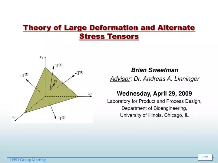
Theory of Large Deformation and Alternate Stress Tensors. Brian Sweetman Advisor : Dr . Andreas A. Linninger Wednesday, April 29, 200 9 Laboratory for Product and Process Design, Department of Bioengineering, University of Illinois, Chicago, IL. Some questions raised last week.

E N D
Theory of Large Deformation and Alternate Stress Tensors Brian Sweetman Advisor: Dr. Andreas A. Linninger Wednesday, April 29, 2009 Laboratory for Product and Process Design, Department of Bioengineering, University of Illinois, Chicago, IL
Some questions raised last week Specific Case Yes! See pg 842 Stewart, Multivariable Calculus, 4th Ed.
What is Stress? A measure of the average amount of force exerted per unit area of the surface on which internal forces act within a deformable body. In other words, it is a measure of the intensity, or internal distribution of the total internal forces acting within a deformable body across imaginary surfaces. These internal forces are produced between the particles in the body as a reaction to external forces applied on the body. External forces are either surface forces or body forces. Because the loaded deformable body is assumed as a continuum, these internal forces are distributed continuously within the volume of the material body, i.e. the stress distribution in the body is expressed as a piecewise continuous function of space coordinates and time. In general, the stress is not uniformly distributed over a cross section of a material body, and consequently the stress at a point on a given area is different than the average stress over the entire area. Therefore, it is necessary to define the stress not at a given area but at a specific point in the body. According to Cauchy, the stress at any point in an object, assumed to be a continuum, is completely defined by nine components of a second order tensor known as the Cauchy stress tensor Stress is defined at a point on a plane (defined by a normal vector)
Some Terms • Continuum Mechanics = Can be used to describe the deformation of a solid body or movement of a fluid • Stress Tensor = Describes the state of stress of a body at a point • Cauchy, 1st Piola Kirchhoff, 2nd Piola Kirchhoff = Stress tensors with different physical interpretations • Deformation Gradient, Displacement Gradient Cauchy Stress Tensor 1st Piola Kirchhoff Stress Tensor 2nd Piola Kirchhoff Stress Tensor
Motivation • The Cauchy stress tensor is a measure of stress in the deformed configuration and does not have terms that relate the body back to a reference configuration. That is why it is not the preferred stress tensor in finite strain theory. • Alternate stress tensors, the Lagrangian/1st Piola Kirchhoff or 2nd Piola-Kirchhoff stress tensors, “are preferred in elasticity where it is assumed that there exists a natural state to which the body would return when it is unloaded”. (Malvern 1969) • The purpose of this presentation is to show how we arrive at these alternate stress tensors and what their physical meaning is. • We will begin by relating the deformed state (volumes and areas) to the reference (undeformed) state
Displacement: Relationship between a point in the reference and deformed configuration Deformed Reference u x X z z y y x x The displacement vector relates a position in the reference configuration to a position in the deformed configuration The above equation represents the relationship between the three coordinates (x, y, z) in a reference and deformed configuration
Deformation Gradient Tensor For a function of two variables, z=f(x,y), we define the differentials dx and dy to be independent variables—they can be given any values. Then the differential dz, also called the total differential, is defined by (Stewart, Multivariable Calculus): z z We want to relate how an infinitesimal material element transforms into the current configuration: y y x x In three spatial directions, we apply the concept of the total derivative in three dimensions to relate the reference configuration to deformed configuration Note that Deformation gradient, F Writing out the indices explicitly we obtain three components of the vector,
Returning to the relationship between a point in the reference and deformed configuration If we differentiate the following set of equations with respect to X1, X2, X3 we obtain the below relations The terms in purple are the same as the terms in the deformation gradient The terms in red are all zero (for example the x coordinate does not depend on the y coordinate for a given point) Deformation gradient Kronecker Delta Displacement gradient
Deformation Gradient Tensor (cont) What does this relation mean? z z y y x x
Relationship between Reference and Deformed Configuration (Volume) z y x Reference (initial, undeformed) configuration Deformed (Current) configuration Scalar triple product How do we relate the vectors in the deformed configuration with the vectors in the reference configuration? From prior slide, we can see that each deformed line, yields the following relations: So,
Relate Reference to Deformed (cont) Because you can move terms around freely when in index notation Continuing relation from prior slide It can be shown (and I have done this) that (If you really want to see the truth of this, you can write out the terms explicitly using the summing convention on repeated indices) Therefore, But we recognize as the undeformed infinitesimal volume element from the prior slide Where J=det F is the ratio of the vol. in the def. config to the vol. in the ref. config. Therefore, This relation allows us to calculate the reference volume in terms of the deformed volume by dividing by the Jacobian: refers to 1 over J (not inverse of a matrix). Remember, J is a scalar. It’s the determinant of the deformation gradient. Note:
Relationship between Reference and Deformed Configuration (Area) We would like to relate an infinitesimal surface area in the deformed configuration to an infinitesimal surface area in the reference configuration. We will use the volume ratio, J, computed in prior slide to derive the area relation Reference configuration Deformed configuration The cross product of above vectors gives the area of the infinitesimal areas in the reference and deformed configuration: We also have for the unit normal vectors: From relations above we obtain:
Relate Reference Area to Deformed Area (cont) We want to relate the reference config to the def config Using the relations from prior slide This makes use of the permutation symbol for cross product Using the above Reference relation and inverse deformation gradient relation (right): Inverse deformation gradient relation So we now have, Multiplying both sides by we obtain,
Area relations (cont) But let us remember this relation Relation from prior slide So we have Where again J-1 is not the inverse of a matrix but simply 1 over J So that we have Multiplying both sides by gives But let us remember this relation So that we have: Quick note This defines a relationship between normal vectors and areas in the reference configuration to normal vectors and areas in the deformed configuration. The formula is called Nanson’s formula
Alternate Stress Tensors: 1st PK Stress “Cauchy’s stress tensor is defined in the deformed configuration and is thus not practical to use for large deformation analysis or experimental measures. Therefore, we need to develop alternative stress tensors.” (BME 456) Based on results from prior slides we are now ready to develop new stress tensors “Consider first the Lagrangian (or 1st PK stress): The 1st Piola-Kirchhoff stress is defined such that the total force resulting from the 1st PK stress multiplied by the normal and area in the reference configuration is the same as the total force resulting from the Cauchy stress times the normal and area in the deformed configuration.” (Google “BME 456” and you will get an amazing tutorial on all this stuff) Now that’s a mouthful, so let’s break it down Total force resulting from the 1st PK stress multiplied by the normal and area in the reference configuration the total force …is the same as the total force resulting from the Cauchy stress times the normal and area in the deformed configuration
Alternate Stress Tensors (cont) Relations from prior slide Nanson’s formula But let us remember this relation Using Nanson’s formula we have: We will now switch the j and k indices (on the right) b/c they are dummy indices Now subtract right side from left Now factor This relation will hold for any arbitrary normal times area So we have Or in matrix form
Relation between Cauchy Stress and 1st PK stress Relation from prior slide “Physical Interpretation: Since the 1st PK stress is defined in the reference configuration, it makes sense that we multiply the Cauchy stress by the inverse of F to map back to the reference configuration. Also, if we divide through the original expression for the 1st PK stress by the reference area, then we get the 1st PK stress traction:” (BME 456) “Physically, this indicates the 1st PK stress is equivalent to dividing the total force in the deformed configuration by the area in the reference configuration. When testing soft tissues, this is the typical stress measurement that is made. We constantly monitor the force via the load cell in the testing system, hence the force in the current deformed configuration, but typically only make a measurement of the cross-sectional area in the reference configuration. Thus, any computed stress is the 1st PK stress.” BME 456 We can write the Cauchy stress tensor in terms of the 1st PK stress Or in matrix form
2nd PK stress (symmetric stress tensor) “One of the difficulties with the 1st PK stress is that it is not a symmetric stress tensor. We can see this because we are multiplying a symmetric stress tensor, the Cauchy stress, with a generally non-symmetric deformation gradient tensor, we will have as a result a non-symmetric tensor. Such non-symmetry makes it difficult to form constitutive models. Therefore, the 2nd PK stress was developed to be a symmetric stress tensor for large deformation. The 2nd PK stress involves one further mapping step between the reference and deformed configuration than the 1st PK stress. As such, it does not have such a straightforward physical interpretation as the 1st PK stress. To develop the total force, dP is transformed from the deformed configuration by using the inverse of the deformation gradient tensor. If we call the transformed force dP’ it may be written as:” (BME 456) “The 2nd PK stress Sij is defined such that the traction force resulting from the 2nd PK stress in the reference configuration multiplied by the area in the reference configuration creates the transformed total force dP':” Another mouthful; we’ll break it down From Malvern
How the 2nd PK Stress and Cauchy Stress are Related Relations from prior slide We therefore have: But let us remember this relation So we then have: “The question is how to replace the deformed area and normal on the right hand side with the reference normal and area on the left hand side so we can make a direct representation. We do this by using Nanson's formula. We obtain”: (BME 456) Nanson’s formula We would like to subtract the right side from the left and have the equation hold for any arbitrary undeformed normal times undeformed area. We do this by changing the index on Nr. Note that indices j, k and r are all repeated in the far right expression; they are dummy indices. So, we may rearrange these indices without changing the meaning of the expression. We will switch the j and r indices to obtain:
How the 2nd PK Stress and Cauchy Stress are Related (cont) Relation from prior slide We subtract the RHS from the LHS (factoring Nj and dA) to obtain: Now because this relation holds for any arbitrary Normal times Area, the expression in the parentheses must be zero and we have the following result: Or in matrix form Thus, we have the 2nd PK stress, Sij defined in terms of the Cauchy stress, inverse deformation gradient and Jacobian has a special name: Kirchhoff Stress Tensor If we want the Cauchy stress in terms of the 2nd PK stress we have: Or in matrix form
How the 1st and 2nd PK Stresses are Related From prior slides we have the following relations: Relationship b/w 1st PK stress and Cauchy Stress Relationship b/w 2nd PK stress and Cauchy Stress Let’s rewrite [1] so that the indices are commensurate with [2] (just replace the i with an r). Now we have the following relation: After rearranging terms This leads to: And the relation seen In Borja paper:
Balance of Linear Momentum in Terms of 1st and 2nd PK Stress It can be shown (see Malvern or search web for “BME 456”) that Bal. of linear momentum in terms of deformed (current) configuration using Cauchy stress tensor or We want to express the balance of linear momentum in terms of the reference configuration as opposed to the deformed configuration. How? By balancing the forces in an integral concept over the whole body. We add up the surface traction forces over the area of the body, the body forces over the volume of the body, and inertia forces also over the volume of the body all in terms of the reference configuration. (paraphrased from BME 456) Here we distinguish between the reference and current configuration by surface traction forces over the area of the body body forces over the volume of the body inertia forces over the volume of the body deviating from the notation used earlier Another explanation is from Malvern: “The equations of motion in the reference state are derived from the condition that the vector sum of the external forces on the material in V, which initially occupied Vo is equal to the rate of change of the momentum. (Note that, although the integrals are over Vo , the forces act on the material in V and the momentum is the momentum in V at time t.)”, pg. 223
Balance of Linear Momentum in Terms of 1st and 2nd PK Stress (cont) Relation from prior slide To combine terms we need to relate everything in terms of a volume integral. We use the divergence theorem for this: [1] becomes Which reduces to: The terms inside must be zero, so we have: This is the stress equilibrium equation with respect to the reference state in terms of the 1st PK stress
Balance of Linear Momentum in Terms of 1st and 2nd PK Stress (cont) Let’s compare the Equations for balance of Linear momentum using the Cauchy stress tensor versus using the 1st PK stress tensor As in Malvern • Density written in terms of the current configuration, ρ • State of body referred to current configuration, x • dv/dt is the material time derivative • Density written in terms of reference configuration, ρo • Stress in body referred to reference configuration, X • “The forces act on the material in V and the momentum is the momentum in V at time t” (Malvern).
Balance of Linear Momentum in Terms of 1st and 2nd PK Stress (cont) Using the relation between 1st and 2nd PK stress derived earlier we write the stress equilibrium equation in terms of the 2nd PK stress, (again, in the reference configuration): Relation between 1st and 2nd PK stress From prior slide So we have:
Continuity Equation in Borja In the limit of incompressible fluid and solid phases, the continuity equation reduces to
Conclusions • Mastering these concepts is essential to understand the Borja paper • Have created a Word file that explains the equations (except the constitutive equations) in Borja. Future Work • Will try to understand the Constitutive Assumptions section of Borja paper.