Download
1 / 60
860 likes | 2.37k Vues
Harmonic Analysis and the Prediction of Tides. Dr. Russell Herman Mathematic and Statistics UNCW.

E N D
Harmonic Analysis and the Prediction of Tides Dr. Russell Herman Mathematic and Statistics UNCW “THE SUBJECT on which I have to speak this evening is the tides, and at the outset I feel in a curiously difficult position. If I were asked to tell what I mean by the Tides I should feel it exceedingly difficult to answer the question. The tides have something to do with motion of the sea.” Lord Kelvin, 1882
Outline • What Are Tides? • Tidal Constituents • Fourier Analysis • Harmonic Analysis • Ellipse Parameters Abstract In this talk we will describe classical tidal harmonic analysis. We begin with the history of the prediction of tides. We then describe spectral analysis and its relation to harmonic analysis. We end by describing current ellipses.
The Importance of Tides Important for commerce and science for thousands of years • Tides produce strong currents • Tidal currents have speeds up to 5m/s in coastal waters • Tidal currents generate internal waves over various topographies. • The Earth's crust “bends” under tidal forces. • Tides influence the orbits of satellites. • Tidal forces are important in solar and galactic dynamics.
Tidal Analysis – Long History • Mariners know tides are related to the moon’s phases • The exact relationship is complicated • Many contributors: • Galileo, Descartes, Kepler, Newton, Euler, Bernoulli, Kant, Laplace, Airy, Lord Kelvin, Jeffreys, Munk and many others • Some of the first computers were developed to predict tides. • Tide-predicting machines were developed and used to predict tidal constituents.
“Rise and fall of the sea is sometimes called a tide; … Now, we find there a good ten feet rise and fall, and yet we are authoritatively told there is very little tide.” “The truth is, the word "tide" as used by sailors at sea means horizontal motion of the water; but when used by landsmen or sailors in port, it means vertical motion of the water.” “One of the most interesting points of tidal theory is the determination of the currents by which the rise and fall is produced, and so far the sailor's idea of what is most noteworthy as to tidal motion is correct: because before there can be a rise and fall of the water anywhere it must come from some other place, and the water cannot pass from place to place without moving horizontally, or nearly horizontally, through a great distance. Thus the primary phenomenon of the tides is after all the tidal current; …” The Tides, Sir William Thomson (Lord Kelvin) – 1882, Evening Lecture To The British Association
Tidal Analysis – Hard Problem! • Important questions remained: • What is the amplitude and phase of the tides? • What is the speed and direction of currents? • What is the shape of the tides? • First, accurate, global maps of deep-sea tides were published in 1994. • Predicting tides along coasts and at ports is much simpler.
Tidal Potential Tides - found from the hydrodynamic equations for a self-gravitating ocean on a rotating, elastic Earth. The driving force - small change in gravity due to relative motion of the moon and sun. Main Forces: • Centripetal acceleration at Earth's surface drives water toward the side of Earth opposite the moon. • Gravitational attraction causes water to be attracted toward the moon. If the Earth were an ocean planet with deep oceans: • There would be two bulges of water on Earth, one on the side facing the moon, one on the opposite side.
Gravitational Potential Terms: Force = gradient of potential 1. No force 2. Constant Force – orbital motion 3. Tidal Potential
Tidal Buldges The tidal potential is symmetric about the Earth-moon line, and it produces symmetric bulges. vertical forces produces very small changes in the weight of the oceans. It is very small compared to gravity, and it can be ignored.
High Tides Allow the Earth to rotate, • An observer in space sees two bulges fixed relative to the Earth-moon line as Earth rotates. • An observer on Earth sees the two tidal bulges rotate around Earth as moon moves one cycle per day. • The moon produces high tides every 12 hours and 25.23 minutes on the equator if it is above the equator. • High tides are not exactly twice per day • the moon rotates around Earth. • the moon is above the equator only twice per lunar month, complicating the simple picture of the tides on an ideal ocean-covered Earth. • the moon's distance from Earth varies since the moon's orbit is elliptical and changing
Lunar and Solar Tidal Forces • Solar tidal forces are similar • Horizontal Components – KS/KM = 0.46051 • Thus, need to know relative positions of sun and moon!
Locating the Sun and the Moon Terminology – Celestial Mechanics • Declination • Vernal Equinox • Right Ascension
Tidal Frequencies jp is latitude at which the tidal potential is calculated, d is declination of moon (or sun) north of the equator, t is the hour angle of moon (or sun).
Solar Motion • The periods of hour angle: solar day of 24hr 0min or lunar day of 24hr 50.47min. • Earth's axis of rotation is inclined 23.45° with respect to the plane of Earth's orbit about the sun. Sun’s declination varies between d= ± 23.45° with a period of one solar year. • Earth's rotation axis precesses with period of 26,000 yrs. • The rotation of the ecliptic plane causes d and the vernal equinox to change slowly • Earth's orbit about the sun is elliptical causing perigee to rotate with a period of 20,900 years. Therefore RSvaries with this period.
Lunar Motion • The moon's orbit lies in a plane inclined at a mean angle of 5.15° relative to the plane of the ecliptic. The lunar declination varies between d = 23.45 ± 5.15° with a period of one tropical month of 27.32 solar days. • The inclination of moon's orbit: 4.97° to 5.32°. • The perigee rotates with a period of 8.85 years. The eccentricity has a mean value of 0.0549, and it varies between 0.044 and 0.067. • The plane of moon's orbit rotates around Earth's axis of with a period of 17.613 years. These processes cause variations in RM
Tidal Potential Periods Lunar Tidal Potential - periods near 14 days, 24 hours, and 12 hours Solar Tidal Potential - periods near 180 days, 24 hours, and 12 hours Doodson (1922) - Fourier Series Expansion using 6 frequencies
Constituent Splitting Doodson's expansion:399 constituents, 100 are long period, 160 are daily, 115 are twice per day, and 14 are thrice per day. Most have very small amplitudes. Sir George Darwin named the largest tides.
How to Obtain Constituents • Fourier (Spectral) Analysis • Harmonic Analysis
Fourier Analysis … In the beginning … • 1742 – d’Alembert – solved wave equation • 1749 – Leonhard Euler – plucked string • 1753 – Daniel Bernoulli – solutions are superpositions of harmonics • 1807 - Joseph Fourier solved heat equation Problems – lead to modern analysis!
Spectral Theory • Fourier Series • Sum of Sinusoidal Functions • Fourier Analysis • Spectrum Analysis • Harmonic Analysis = +
Reconstruction FourierExpansion: Power Spectrum Comparison between f(x) and F(x)
Analog Signals • Analog Signals • Continuous in time and frequency • Infinite time and frequency domains • Described by Fourier Transform • Real Signals • Sampled at discrete times • Finite length records • Leads to discrete frequencies on finite interval • Described by Discrete Fourier Transform
DFT – Discrete Fourier Transform Sampled Signal: and
Matlab Implementation y=[7.6 7.4 8.2 9.2 10.2 11.5 12.4 13.4 13.7 11.8 10.1 ... 9.0 8.9 9.5 10.6 11.4 12.9 12.7 13.9 14.2 13.5 11.4 10.9 8.1]; N=length(y); % Compute the matrices of trigonometric functions p=1:N/2+1; n=1:N; C=cos(2*pi*n'*(p-1)/N); S=sin(2*pi*n'*(p-1)/N); % Compute Fourier Coefficients A=2/N*y*C; B=2/N*y*S; A(N/2+1)=A(N/2+1)/2; % Reconstruct Signal - pmax is number of frequencies used in increasing order pmax=13; ynew=A(1)/2+C(:,2:pmax)*A(2:pmax)'+S(:,2:pmax)*B(2:pmax)'; % Plot Data plot(y,'o') % Plot reconstruction over data hold on plot(ynew,'r') hold off
DFT Example Monthly mean surface temperature (oC) on the west coast of Canada January 1982-December 1983 (Emery and Thompson)
Harmonic Analysis • Consider a set of data consisting of N values at equally spaced times, • We seek the best approximation using M given frequencies. • The unknown parameters in this case are the A’s and B’s.
Linear Regression • Minimize • Normal Equations
Matlab Implementation – DZ=Y y=[7.6 7.4 8.2 9.2 10.2 11.5 12.4 13.4 13.7 11.8 10.1 ... 9.0 8.9 9.5 10.6 11.4 12.9 12.7 13.9 14.2 13.5 11.4 10.9 8.1]; N=length(y); % Number of Harmonics Desired and frequency dt M=2; f=1/12*(1:M); T=24; alpha=f*T; % Compute the matrices of trigonometric functions n=1:N; C=cos(2*pi*alpha'*n/N); S=sin(2*pi*alpha'*n/N); c_row=ones(1,N)*C'; s_row=ones(1,N)*S'; D(1,1)=N; D(1,2:M+1)=c_row; D(1,M+2:2*M+1)=s_row; D(2:M+1,1)=c_row'; D(M+2:2*M+1,1)=s_row'; D(2:M+1,2:M+1)=C*C'; D(M+2:2*M+1,2:M+1)=S*C'; D(2:M+1,M+2:2*M+1)=C*S'; D(M+2:2*M+1,M+2:2*M+1)=S*S'; yy(1,1)=sum(y); yy(2:M+1)=y*C'; yy(M+2:2*M+1)=y*S'; z=D^(-1)*yy';
Harmonic Analysis Example Frequencies 0.0183 cpmo, 0.167 cpmo
Example 2 data = DLMREAD('tidedat1.txt'); N=length(data); t=data(1:N,1); % time r=data(1:N,2); % height ymean=mean(r); % calculate average ynorm=r-ymean; % subtract out average y=ynorm'; % height' dt=t(2)-t(1); T=t(N); % Number of Harmonics Desired and frequency dt M=8; TideNames=['M2','N2','K1','S2','O1','P1','K2','Q1']; TidePeriods=[12.42 12.66 23.93 12 25.82 24.07 11.97 26.87]; f=1./TidePeriods;
Periodogram - Period Names =['M2', 'N2', 'K1', 'S2', 'O1', 'P1', 'K2', 'Q1']; Periods=[12.42 12.66 23.93 12 25.82 24.07 11.97 26.87];
Current Analysis • Horizontal Currents are two dimensional • One performs the harmonic analysis on vectors • The results for each constituent are combined and reported using ellipse parameters