Download
1 / 37
380 likes | 533 Vues
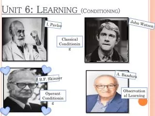
Chapter 6 Learning Through Conditioning. Classical conditioning. Pavlov’s Demonstration Terminology Unconditioned Stimulus (UCS) Conditioned Stimulus (CS) Unconditioned Response (UCR) Conditioned Response (CR). Figure 6.1

E N D
Classical conditioning • Pavlov’s Demonstration • Terminology • Unconditioned Stimulus (UCS) • Conditioned Stimulus (CS) • Unconditioned Response (UCR) • Conditioned Response (CR)
Figure 6.1 Classical conditioning apparatus. An experimental arrangement similar to the one depicted here (taken from Yerkes & Morgulis, 1909) has typically been used in demonstrations of classical conditioning, although Pavlov’s original setup (see inset) was quite a bit simpler. The dog is restrained in a harness. A tone is used as the conditioned stimulus (CS), and the presentation of meat powder is used as the unconditioned stimulus (UCS). The tube inserted into the dog’s salivary gland allows precise measurement of its salivation response. The pen and rotating drum of paper on the left are used to maintain a continuous record of salivary flow. (Inset) The less elaborate setup that Pavlov originally used to collect saliva on each trial is shown here (Goodwin, 1991).
Figure 6.2 The sequence of events in classical conditioning. Moving from top to bottom, this series of diagrams outlines the sequence of events in classical conditioning, using Pavlov’s original demonstration as an example. As we encounter other examples of classical conditioning throughout the book, we will see many diagrams like the one in the fourth panel, which summarizes the process.
Figure 6.3 Classical conditioning of a fear response. Many emotional responses that would otherwise be puzzling can be explained by classical conditioning. In the case of one woman’s bridge phobia, the fear originally elicited by her father’s scare tactics became a conditioned response to the stimulus of bridges.
Classical Conditioning: Terminology Continued • Trial = pairing of UCS and CS • Acquisition = initial stage in learning • Stimulus contiguity = occurring together in time and space • 3 types of Classical Conditioning • Simultaneous conditioning: CS and UCS begin and end together • Short-delayed conditioning: CS begins just before the UCS, end together • Trace conditioning: CS begins and ends before UCS is presented
Figure 6.9 Temporal relations of stimuli in classical conditioning. The effects of classical conditioning depend in part on the timing of the stimuli. Three ways of pairing the CS and UCS are diagrammed here. The most effective arrangement is short-delayed conditioning, in which the CS begins just before the UCS and stops at the same time as the UCS.
Processes in Classical Conditioning • Extinction • Spontaneous Recovery • Stimulus Generalization • Discrimination • Higher-order conditioning
Figure 6.6 Classical conditioning of immunosuppression. When a neutral stimulus is paired with a drug that chemically causes immunosuppression, it can become a CS that elicits immunosuppression on its own. Thus, even the immune response can be influenced by classical conditioning.
Figure 6.12 Generalization gradients. In a study of stimulus generalization, an organism is typically conditioned to respond to a specific CS, such as a 1200 hertz tone, and then tested with similar stimuli, such as other tones between 400 and 2000 hertz. Graphs of the organisms’ responding are called generalization gradients. The graphs normally show, as depicted here, that generalization declines as the similarity between the original CS and the new stimuli decreases. When an organism gradually learns to discriminate between a CS and similar stimuli, the generalization gradient tends to narrow around the original CS.
Figure 6.13 Higher-order conditioning. Higher-order conditioning is a two-phase process. In the first phase, a neutral stimulus (such as a tone) is paired with an unconditioned stimulus (such as meat powder) until it becomes a conditioned stimulus that elicits the response originally evoked by the UCS (such as salivation). In the second phase, another neutral stimulus (such as a red light) is paired with the previously established CS, so that it also acquires the capacity to elicit the response originally evoked by the UCS.
Operant Conditioning or Instrumental Learning • Edward L. Thorndike (1913) – the law of effect • B.F. Skinner (1953) – principle of reinforcement • Operant chamber • Emission of response • Reinforcement contingencies • Cumulative recorder
Figure 6.14 The learning curve of one of Thorndike’s cats. The inset shows one of Thorndike’s puzzle boxes. The cat had to perform three separate actions to escape the box, including depressing the pedal on the right. The learning curve shows how the cat’s escape time declined gradually over a number of trials.
Figure 6.16 Skinner box and cumulative recorder. (a) This diagram highlights some of the key features of an operant chamber, or Skinner box. In this apparatus designed for rats, the response under study is lever pressing. Food pellets, which may serve as reinforcers, are delivered into the food cup on the right. The speaker and light permit manipulations of visual and auditory stimuli, and the electric grid gives the experimenter control over aversive consequences (shock) in the box.
Launch Video Figure 6.17 A graphic portrayal of operant responding. The results of operant conditioning are often summarized in a graph of cumulative responses over time. The insets magnify small segments of the curve to show how an increasing response rate yields a progressively steeper slope (bottom); a high, steady response rate yields a steep, stable slope (middle); and a decreasing response rate yields a progressively flatter slope (top).
Basic Processes in Operant Conditioning • Acquisition • Shaping • Extinction • Stimulus Control • Generalization • Discrimination
Fig 6.18 Operant conditioning shapes behavior as a sculptor shapes a lump of clay.
Reinforcement: Consequences that Strengthen Responses • Delayed Reinforcement • Longer delay, slower conditioning • Primary Reinforcers • Satisfy biological needs • Secondary Reinforcers • Conditioned reinforcement
Schedules of Reinforcement • Continuous reinforcement • Intermittent (partial) reinforcement • Ratio schedules • Fixed • Variable • Interval schedules • Fixed • Variable
Figure 6.19 Schedules of reinforcement and patterns of response. Each type of reinforcement schedule tends to generate a characteristic pattern of responding. In general, ratio schedules tend to produce more rapid responding than interval schedules (note the steep slopes of the FR and VR curves). In comparison to fixed schedules, variable schedules tend to yield steadier responding (note the smoother lines for the VR and VI schedules on the right) and greater resistance to extinction.
Consequences: Reinforcement and Punishment • Increasing a response: • Positive reinforcement = response followed by rewarding stimulus • Negative reinforcement = response followed by removal of an aversive stimulus • Escape learning • Avoidance learning • Decreasing a response: • Punishment • Problems with punishment
Figure 6.21 Positive reinforcement versus negative reinforcement. In positive reinforcement, a response leads to the presentation of a rewarding stimulus. In negative reinforcement, a response leads to the removal of an aversive stimulus. Both types of reinforcement involve favorable consequences and both have the same effect on behavior: The organism’s tendency to emit the reinforced response is strengthened.
Figure 6.22 Escape and avoidance learning. (a) Escape and avoidance learning are often studied with a shuttle box like that shown here. Warning signals, shock, and the animal’s ability to flee from one compartment to another can be controlled by the experimenter. (b) According to Mowrer’s two-process theory, avoidance begins because classical conditioning creates a conditioned fear that is elicited by the warning signal (panel 1). Avoidance continues because it is maintained by operant conditioning (panel 2). Specifically, the avoidance response is strengthened through negative reinforcement, since it leads to removal of the conditioned fear.
Figure 6.23 Comparison of negative reinforcement and punishment. Although punishment can occur when a response leads to the removal of a rewarding stimulus, it more typically involves the presentation of an aversive stimulus. Students often confuse punishment with negative reinforcement because they associate both with aversive stimuli. However, as this diagram shows, punishment and negative reinforcement represent opposite procedures that have opposite effects on behavior.
Changes in Our Understanding of Conditioning • Biological Constraints on Conditioning • Instinctive Drift • Conditioned Taste Aversion • Preparedness and Phobias • Cognitive Influences on Conditioning • Signal relations • Response-outcome relations
Figure 6.24 Conditioned taste aversion. Taste aversions can be established through classical conditioning, as in the “sauce béarnaise syndrome.” However, as the text explains, taste aversions can be acquired in ways that seem to violate basic principles of classical conditioning.
Figure 6.25 Garcia and Koelling’s research on conditioned taste aversion. In a landmark series of studies, Garcia and Koelling (1966) demonstrated that some stimulus-response associations are much easier to condition than others. (a) Their procedure allowed them to pair a taste stimulus (saccharin-flavored water) with visual and auditory stimuli (a bright light and noisy buzzer), and/or pain-inducing shock or nausea-inducing radiation. (b) They found that taste-nausea associations were acquired easily, as were associations between auditory-visual stimuli and pain, whereas other associations were difficult to acquire. As your text discusses, they explained their findings in terms of evolutionary considerations.
Observational Learning: Basic Processes • Albert Bandura (1977, 1986) • Observational learning • Vicarious conditioning • 4 key processes • attention • retention • reproduction • motivation • acquisition vs performance
Figure 6.26 Observational learning. In observational learning, an observer attends to and stores a mental representation of a model’s behavior (example: assertive bargaining) and its consequences (example: a good buy on a car). If the observer sees the modeled response lead to a favorable outcome, the observer’s tendency to emit the modeled response will be strengthened.
Figure 6.27 Steps in a self-modification program. This flowchart provides an overview of the steps necessary to execute a self-modification program.