Download
1 / 118
1.63k likes | 2.39k Vues
II. The Multivariate Normal Distribution.

E N D
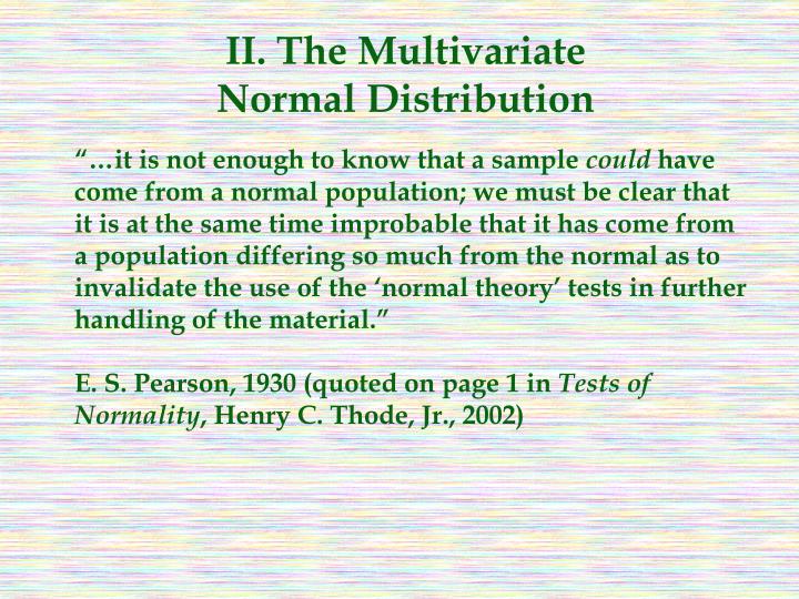
II. The Multivariate Normal Distribution “…it is not enough to know that a sample could have come from a normal population; we must be clear that it is at the same time improbable that it has come from a population differing so much from the normal as to invalidate the use of the ‘normal theory’ tests in further handling of the material.” E. S. Pearson, 1930 (quoted on page 1 in Tests of Normality, Henry C. Thode, Jr., 2002)
A. Review of the Univariate Normal Distribution Normal Probability Distribution - expresses the probabilities of outcomes for a continuous random variable x with a particular symmetric and unimodal distribution. This density function is given by where = mean = standard deviation = 3.14159… e = 2.71828…
but the probability is given by This looks like a difficult integration problem! Will I have to integrate this function every time I want to calculate probabilities for some normal random variable?
Characteristics of the normal probability distribution are: - there are an infinite number of normal distributions, each defined by their unique combination of the mean and standard deviation - determines the central location and determines the spread or width - the distribution is symmetric about - it is unimodal - = Md = Mo - it is asymptotic with respect to the horizontal axis - the area under the curve is 1.0 - it is neither platykurtic nor leptokurtic - it follows the empirical rule:
Normal distributions with the same mean but different standard deviations:
Normal distributions with the same standard deviation but different means:
The Standard Normal Probability Distribution - the probability distribution associated with any normal random variable (usually denoted z) that has = 0 and = 1. There are tables that can be used to obtain the results of the integration for thestandard normal random variable.
Some of the tables work from the cumulative standard normal probability distribution (the probability that a random value selected from the standard normal random variable falls between – and some given value b > 0, i.e., P(- z b)) There are tables that give the results of the integration (Table 1 of the Appendices in J&W).
Let’s focus on a small part of the Cumulative Standard Normal Probability Distribution Table Example: for a standard normal random variable z, what is the probability that z is between - and 0.43?
Example: for a standard normal random variable z, what is the probability that z is between 0 and 2.0? 2.0
Again, looking at a small part of the Cumulative Standard Normal Probability Distribution Table, we find the probability that a standard normal random variable z is between - and 2.00?
Example: for a standard normal random variable z, what is the probability that z is between 0 and 2.0? Area of Probability = 0.9772 – 0.5000 = 0.4772 Area of Probability = 0.5000 { } 2.0
What is the probability that z is at least 2.0? Area of Probability = 1.0000 - 0.9772 = 0.0228 { 2.0
What is the probability that z is between -1.5 and 2.0? Area of Probability = 0.4772 } -1.5 2.0
Again, looking at a small part of the Cumulative Standard Normal Probability Distribution Table, we find the probability that a standard normal random variable z is between - and 1.50?
What is the probability that z is between -1.5 and 2.0? Area of Probability = 0.5000 - 0.0668 = 0.4332 Area of Probability = 0.4772 } } -1.5 2.0
Notice we could find the probability that z is between -1.5 and 2.0 another way! Area of Probability = 1.0000 - 0.9332 = 0.0668 Area of Probability = 0.9772 } } -1.5 2.0
There are often multiple ways to use the Cumulative Standard Normal Probability Distribution Table to find the probability that a standard normal random variable z is between two given values! How do you decide which to use? - Do what you understand (make yourself comfortable) and - DRAW THE PICTURE!!!
Notice we could also calculate the probability that z is between -1.5 and 2.0 yet another way! Area of Probability = 0.9332 - 0.5000 = 0.4332 Area of Probability = 0.4772 } } -1.5 2.0
What is the probability that z is between -1.5 and -2.0? Area of Probability = 0.5000 - 0.0228 = 0.4772 Area of Probability = 0.4772 – 0.4332 = 0.0440 } Area of Probability = 0.4332 } } -2.0 -1.5
What is the probability that z is exactly 1.5? Area of Probability = 0.9332 } 1.5 (why?)
Other tables work from the half standard normal probability distribution (the probability that a random value selected from the standard normal random variable falls between 0 and some given value b > 0, i.e., P(0 z b)) There are tables that give the results of the integration as well.
Let’s focus on a small part of the Standard Normal Probability Distribution Table Example: for a standard normal random variable z, what is the probability that z is between 0 and 0.43?
Example: for a standard normal random variable z, what is the probability that z is between 0 and 2.0? 2.0
Again, looking at a small part of the Standard Normal Probability Distribution Table, we find the probability that a standard normal random variable z is between 0 and 2.00?
Example: for a standard normal random variable z, what is the probability that z is between 0 and 2.0? Area of Probability = 0.4772 } 2.0
What is the probability that z is at least 2.0? Area of Probability = 0.5000 - 0.4772 = 0.0228 { 2.0
What is the probability that z is between -1.5 and 2.0? Area of Probability = 0.4772 } -1.5 2.0
Again, looking at a small part of the Standard Normal Probability Distribution Table, we find the probability that a standard normal random variable z is between 0 and –1.50?
What is the probability that z is between -1.5 and 2.0? Area of Probability = 0.4332 Area of Probability = 0.4772 } } -1.5 2.0
What is the probability that z is between -1.5 and -2.0? Area of Probability = 0.4772 Area of Probability = 0.4772 – 0.4332 = 0.0440 } Area of Probability = 0.4332 } } -2.0 -1.5
What is the probability that z is exactly 1.5? Area of Probability = 0.4332 } 1.5 (why?)
z-Transformation - mathematical means by which any normal random variable with a mean and standard deviation can be converted into a standard normal random variable. - to make the mean equal to 0, we simply subtract from each observation in the population - to then make the standard deviation equal to 1, we divide the results in the first step by The resulting transformation is given by
Example: for a normal random variable x with a mean of 5 and a standard deviation of 3, what is the probability that x is between 5.0 and 7.0? Area of Probability } 7.0 0.0 z
Using the z-transformation, we can restate the problem in the following manner: then use the standard normal probability table to find the ultimate answer:
which graphically looks like this: Area of Probability = 0.2486 } 7.0 0.0 0.67 z
Why is the normal probability distribution considered so important? - many random variables are naturally normally distributed - many distributions, such as the Poisson and the binomial, can be approximated by the normal distribution (Central Limit Theorem) - the distribution of many statistics, such as the sample mean and the sample proportion, are approximately normally distributed if the sample is sufficiently large (also Central Limit Theorem)
B. The Multivariate Normal Distribution The univariate normal distribution has a generalized form in p dimensions – the p-dimensional normal density function is squared generalized distance from x to m where - xi , i = 1,…,p. This p-dimensional normal density function is denoted by Np(m,S) where ~ ~ ~ ~
The simplest multivariate normal distribution is the bivariate (2 dimensional) normal distribution, which has the density function squared generalized distance from x to m where - xi , i = 1, 2. This 2-dimensional normal density function is denoted by N2(m,S) where ~ ~ ~ ~
We can easily find the inverse of the covariance matrix (by using Gauss-Jordan elimination or some other technique): Now we use the previously established relationship to establish that
which means that we can rewrite the bivariate normal probability density function as
Graphically, the bivariate normal probability density function looks like this: contours X2 X1 All points of equal density are called a contour, defined for p-dimensions as all x such that ~
The contours form concentric ellipsoids centered at m with axes ~ X2 contour for constant c f(X1, X2) X1 where
The general form of contours for a bivariate normal probability distribution where the variables have equal variance (s11 = s22) is relative easy to derive: First we need the eigenvalues of S ~
- for a positive covariance s12, the first eigenvalue and its associated eigenvector lie along the 450 line running through the centroid m: ~ X2 contour for constant f(X1, X2) X1 What do you suppose happens when the covariance is negative? Why?
- for a negative covariance s12, the second eigenvalue and its associated eigenvector lie at right angles to the 450 line running through the centroid m: ~ X2 contour for constant f(X1, X2) X1 What do you suppose happens when the covariance is zero? Why?